Ranking Queries: Focus on retrieving the top- objects from a dataset according to a scoring function or proximity to a target (e.g., -nearest neighbors). These queries are essential in applications like search engines, e-commerce, and recommender systems, where users seek the most relevant or preferred results rather than exhaustive listings. Ranking queries can be based on single or multiple attributes, and may involve complex joins across multiple tables.
Rank Aggregation: Addresses the challenge of combining multiple ranked lists into a single consensus ranking. Classic methods include:
Borda’s Method: Assigns points based on rank positions; the candidate with the lowest total penalty wins.
Condorcet’s Method: Seeks a candidate who beats all others in pairwise comparisons.
Aggregation Metrics:
Kendall Tau Distance: Counts pairwise swaps needed to align rankings (NP-complete to optimize).
Spearman’s Footrule: Sums absolute rank differences (tractable in polynomial time).
MedRank Algorithm: Efficiently combines opaque rankings (where only order is known) by selecting items with median ranks across lists; instance-optimal for sorted access.
Top- Query Algorithms:
Naïve Approach: Computes scores for all tuples, sorts them, and selects the top-; simple but inefficient for large datasets.
Fagin’s Algorithm (FA): Uses parallel sorted access and random access to combine ranked lists with a monotone scoring function; stops when common objects are found. General-purpose but not instance-optimal.
Threshold Algorithm (TA): Instance-optimal for monotone scoring functions using both sorted and random access. Maintains a dynamic threshold to determine when the top- set is final, minimizing unnecessary accesses.
No Random Access (NRA): Designed for environments where random access is not possible. Maintains lower and upper bounds for each object’s score and stops when it is certain that the current top- cannot be beaten. Instance-optimal among sorted-access-only algorithms.
Top- Joins: Extend ranking queries to multi-table joins, where the global score is computed from attributes across relations. Efficient algorithms are needed to avoid computing all possible join results, especially in many-to-many joins.
Scoring Functions: Combine normalized attribute scores into a global score for each object. Common functions include:
SUM/AVG: Equal weight to all attributes.
WSUM (Weighted Sum): Attributes weighted by importance.
MIN/MAX: Focus on the worst/best attribute value.
Iso-score Curves: Visualize sets of points with equal global scores in attribute space, aiding in understanding how scoring functions partition the data.
-Nearest Neighbors (k-NN): A special case of ranking queries where objects are ranked by their distance to a target point in multi-dimensional space. Distance functions (e.g., Euclidean, Manhattan, Chebyshev) can be weighted to reflect attribute importance.
Skyline Queries: Identify all non-dominated tuples (Pareto-optimal set) in a dataset, where a tuple is non-dominated if no other tuple is better in all dimensions and strictly better in at least one. Useful for multi-criteria decision-making when user preferences are unknown or not explicitly specified.
Algorithms:
Block Nested Loop (BNL): Compares each tuple to current skyline candidates; simple but time.
Sort-Filter-Skyline (SFS): Sorts tuples by a monotone function, then filters for skyline points in time.
k-Skyband: Generalizes the skyline by including tuples dominated by fewer than others, allowing control over result size and granularity.
Comparison: Ranking vs. Skyline Queries:
Ranking Queries: Best when user preferences are well-defined and a concise, prioritized result set is needed. Allow explicit trade-offs among attributes via scoring functions and control over result size.
Skyline Queries: Best for exploratory analysis, providing a comprehensive overview of all potentially optimal options without requiring explicit preference weights. Useful for understanding trade-offs and the structure of the data, but may return large result sets in high-dimensional or anti-correlated data.
Key Takeaways:
Efficient top- and skyline query processing is crucial for modern data-driven applications.
Choice of algorithm and query type depends on data size, access patterns, scoring function properties, and whether user preferences are known.
Understanding the strengths and limitations of each approach enables better system design and user experience in multi-criteria search and decision support.
In business applications, the majority of queries are designed to yield exact results. These results are often organized in a specific order to improve accessibility and readability, but there is no inherent preference among the outcomes—each result holds equal relevance and importance. This contrasts with consumer applications, where certain queries necessitate ranking the results based on a notion of “preferability.” In such cases, the simultaneous optimization of various criteria is often required.
For example, objects in a dataset may be described by multiple attributes, and a general problem arises: how to identify the best objects based on a defined measure of "goodness."
Example
Consider practical scenarios: search engines rank web pages according to relevance, e-commerce platforms prioritize product listings based on user preferences, and recommender systems suggest items tailored to individual tastes.
In machine learning, this principle appears in tasks such as finding the -nearest neighbors. Here, given data points in a -dimensional metric space and a query point , the objective is to identify the points closest to . This approach underpins classification algorithms, feature selection, and various other domains.
To address such problems, two major approaches are commonly employed: ranking queries and skyline queries.
Ranking queries involve selecting the top objects based on a scoring function, such as relevance or utility.
In contrast, skyline queries identify a set of non-dominated objects—those that are not outperformed by any other object in all criteria.
These approaches have broad applicability in both academic research and real-world systems, forming the backbone of methods to rank, classify, and filter information effectively.
Historical Perspective: Rank Aggregation
The challenge of rank aggregation—combining multiple ranked lists to produce a consensus ranking—has been a focus of study for centuries, primarily within the realm of social choice theory. Early contributions date back to Ramon Llull in the 13th century, who introduced methods for aggregating preferences. Later, Borda (1770) and the Marquis de Condorcet (1785) proposed more systematic methods to tackle this problem.
Rank aggregation addresses a fundamental question: given candidates and voters, how can one determine the overall ranking of candidates based on the preferences of all voters? Unlike modern scoring systems, early approaches did not assign visible scores to candidates but instead relied solely on ordinal rankings. Key problems include identifying the “best” candidate and resolving inconsistencies that arise when individual rankings conflict—a hallmark of Condorcet’s paradox, where collective preferences can form cycles.
Borda’s and Condorcet’s Proposals
Borda and Condorcet proposed two influential methods for aggregating preferences in elections, each rooted in distinct philosophical principles.
Borda’s Method organizes elections based on the principle of order of merit. In this system, candidates receive points corresponding to their rank in each voter’s preference list. Specifically, the first-place candidate receives 1 point, the second-place candidate receives 2 points, and so on, up to th place, which receives points. The penalty for each candidate is the sum of their points across all voters’ rankings. The candidate with the lowest penalty is declared the Borda winner, emphasizing overall favorability across the electorate rather than dominance in head-to-head comparisons.
In contrast, Condorcet’s Method focuses on pairwise majority elections. A candidate is considered the Condorcet winner if they defeat every other candidate in a direct comparison based on majority rule. This criterion captures the idea of dominance but introduces the possibility of cyclic preferences, where no single candidate wins all pairwise contests. In such cases, the Condorcet winner does not exist, revealing the limitations of majority rule in ranking aggregation.
Example: Comparing Borda and Condorcet Winners
Consider the following voter preferences, where the ranks are ordered by columns:
Voter
1
2
3
4
5
6
7
8
9
10
A
1
1
1
1
1
1
3
3
3
3
C
2
2
2
2
2
2
1
1
1
1
B
3
3
3
3
3
3
2
2
2
2
Using Borda’s scoring, we calculate the penalties:
Here, candidate C has the lowest penalty and is the Borda winner.
Using Condorcet’s criterion, we compare candidates in pairwise elections:
A defeats B (6 votes to 4).
A defeats C (6 votes to 4).
Thus, A is the Condorcet winner, as it wins against both B and C in direct comparisons. This highlights a potential divergence: while C is the Borda winner, A is the Condorcet winner, illustrating the differing priorities of the two methods.
Approaches to Rank Aggregation
Rank aggregation remains central to various applications, from elections to search engine optimization.
Definition
A common mathematical formulation seeks a consensus ranking that minimizes the total distance to the initial rankings .
Two widely used metrics for comparing rankings are:
Kendall Tau Distance (): This measures the number of pairwise swaps needed to transform one ranking into another.
For example, bubble sort’s count of exchanges to sort into provides this distance.
While intuitive, finding an exact solution to minimize Kendall tau distance is computationally hard (NP-complete).
Spearman’s Footrule Distance (): This sums the absolute differences between the ranks of corresponding items in and . Unlike Kendall tau, Spearman’s footrule distance is computationally tractable (PTIME) and can be efficiently approximated. This makes it practical for large-scale problems, where median ranking serves as a useful heuristic.
The computational challenges in rank aggregation depend on the metric used:
For Kendall tau distance, finding an optimal aggregation is NP-complete, making it infeasible for large datasets without approximation techniques.
For Spearman’s footrule, efficient polynomial-time solutions exist, with approximations available for even faster results in high-dimensional cases.
Combining Opaque Rankings with MedRank
When dealing with ranked lists where only the position of elements matters—without access to associated scores—specific techniques like MedRank can be employed to combine rankings effectively. MedRank, based on the concept of the median, provides an approximate solution to Footrule-optimal aggregation. This method is particularly useful when rankings are opaque, such as hotel rankings based on price, rating, and distance, where only the order of items in each list is known.
Algorithm
The algorithm takes as input:
An integer , representing the desired number of top elements.
ranked lists , each containing elements.
Output: The top elements based on median ranking.
Steps:
Sorted Access: MedRank performs one sorted access at a time on each list, retrieving elements sequentially.
Selection Criteria: It continues until there are elements that appear in more than of the lists.
Output: These elements are returned as the top , with their rank determined by their median positions across the lists.
Example: Ranking Hotels
Consider three ranked lists of hotels based on different criteria—price, rating, and distance. The goal is to find the top 3 hotels using median ranking.
Price
Rating
Distance
1
Ibis
Crillon
Le Roch
2
Etap
Novotel
Lodge In
3
Novotel
Sheraton
Ritz
4
Mercure
Hilton
Lutetia
5
Hilton
Ibis
Novotel
6
Sheraton
Ritz
Sheraton
7
Crillon
Lutetia
Mercure
To determine the top 3 hotels, MedRank accesses elements in order from each list and calculates their median ranks:
Novotel: Positions across the lists → Median rank .
Hilton: Positions → Median rank .
Ibis: Positions → Median rank .
The algorithm stops when it identifies the top 3 elements based on their median ranks. Here, the depth, or the maximum number of sorted accesses on any list, is 5. Ideally, when all median ranks are distinct, the result matches the Footrule-optimal aggregation.
MedRank is instance-optimal for combining rankings accessed in sorted order. Instance optimality means that for any given input:
MedRank’s execution cost is at most a constant factor higher than the execution cost of any other algorithm tailored to that input.
MedRank guarantees the best performance (up to a constant factor) across all possible instances where rankings are accessed sequentially.
This is a stronger guarantee than average-case or worst-case optimality. For instance:
Binary search is worst-case optimal because it performs comparisons, unlike sequential search, which takes in the worst case.
However, binary search is not instance-optimal, as its performance can be significantly worse than a specialized algorithm for specific inputs.
MedRank’s optimality ratio, , is 2.
This means that its execution cost is at most twice the cost of any other algorithm designed for the same instance.
While not optimal in all scenarios, this property makes MedRank robust and efficient for practical use cases.
MedRank’s utility lies in its simplicity and effectiveness for aggregating rankings when only positional information is available. Its ability to approximate Footrule-optimal aggregation efficiently makes it applicable in various domains, such as:
Recommender systems: Combining user preferences across categories.
Multi-criteria decision-making: Selecting top options based on multiple factors.
Search engines: Aggregating rankings from different sources without explicit scoring.
Ranking Queries (top-k Queries)
Ranking queries aim to retrieve the top best results from a potentially vast dataset, where “best” is determined by relevance, importance, or interest.
This is crucial in applications such as e-commerce, web search, multimedia systems, and scientific databases, where users seek the most relevant answers rather than exhaustive listings.
The Naïve Approach to Ranking
A common, straightforward method for ranking is to use a scoring function, which assigns numerical scores to each tuple based on its attributes.
Algorithm
Taking as input the cardinality , a dataset , and a scoring function , to obtain the highest-scored tuples with respect to , the naive approach is as follows:
Compute the score for every tuple in the dataset .
Sort all tuples by their scores in descending order.
Select the top tuples as the result.
Example
For example, could combine a basketball player’s statistics.
Name
Points
Rebounds
Score ()
Shaquille O’Neal
1669
760
2429
Tracy McGrady
2003
484
2487
Kobe Bryant
1819
392
2211
Yao Ming
1465
669
2134
Dwyane Wade
1854
397
2251
While simple, this approach becomes computationally expensive for large datasets because it requires sorting all tuples, which has a complexity of . This inefficiency is compounded when the query involves joining multiple tables, especially if the join is many-to-many.
SQL offers tools to handle ranking queries, though historically these have evolved over time:
Sorting: Achieved through the ORDER BY clause.
Limiting results: Only natively supported in SQL since the SQL:2008 standard using FETCH FIRST k ROWS ONLY. Earlier databases relied on non-standard syntaxes like LIMIT k (PostgreSQL, MySQL) or SELECT TOP k (SQL Server).
Example
For example, consider ranking used cars by a weighted score
Query A filters cars by price () and orders the results:
SELECT *FROM UsedCarsTable WHERE Vehicle = 'Audi/A4' AND Price <= 21000ORDER BY 0.8*Price + 0.2*Miles;
This query is efficient but may exclude relevant results that slightly exceed the price limit but have better mileage (near-miss problem).
Query B removes the price filter, returning all cars and ordering them by their weighted score:
SELECT *FROM UsedCarsTable WHERE Vehicle = 'Audi/A4'ORDER BY 0.8*Price + 0.2*Miles;
While this query ensures no potentially relevant results are missed, it risks overwhelming users with an exhaustive list of results (information overload problem).
Two primary abilities are required to perform efficient and relevant ranking queries:
Sorting by Scores: Implemented through the ORDER BY clause.
Limiting the Result Set: Controlled by clauses like LIMIT or FETCH FIRST k ROWS ONLY.
However, predefined filters (e.g., price limits) can create trade-offs:
Near-Miss Problem: Strict filters may exclude near-optimal results.
Information Overload: Broad queries may return too many results to be useful.
Weighting factors like (price) and (mileage) reflect user preferences and enable fine-tuned ranking. The weights normalize different attributes, allowing multi-dimensional comparisons.
Given the inefficiencies of the naive approach, more sophisticated techniques are often employed to improve performance, such as:
Indexing: Creating indexes on frequently queried attributes can reduce query time.
Approximate Methods: Sampling or heuristic-based algorithms may reduce computation time while maintaining acceptable accuracy.
Incremental Approaches: Algorithms that generate results progressively, stopping as soon as the top tuples are identified, avoid processing the entire dataset.
Semantics of Top-k Queries
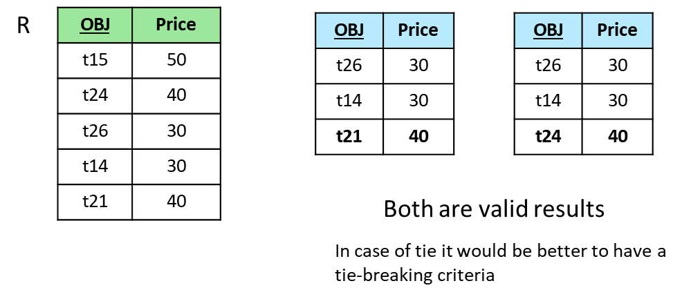
Top- queries aim to retrieve the most relevant tuples according to a scoring function or ordering criterion. The semantics allow for non-determinism if multiple sets of tuples equally satisfy the ordering criteria. The first tuples that meet the criteria are part of the result, but the selection among equally ranked tuples may vary.
For example, given:
SELECT * FROM R ORDER BY Price FETCH FIRST 3 ROWS ONLY
If multiple tuples have identical prices that qualify them for the th position, any of these tuples can appear in the result, leading to non-deterministic behavior.
Examples of Top- Queries
Best NBA Player by Points and Rebounds
SELECT *FROM NBA ORDER BY Points + Rebounds DESCFETCH FIRST 1 ROW ONLY;
Two Cheapest Chinese Restaurants
SELECT *FROM RESTAURANTS WHERE Cuisine = 'Chinese'ORDER BY Price FETCH FIRST 2 ROWS ONLY;
Top 5 Audi/A4 by Weighted Score of Price and Mileage
SELECT *FROM USEDCARS WHERE Vehicle = 'Audi/A4'ORDER BY 0.8*Price + 0.2*Miles FETCH FIRST 5 ROWS ONLY;
Top- query evaluation depends on two key factors:
Query Type: Single relation, multi-relation joins, or aggregated results.
Access Paths: Availability of indexes for ranking attributes.
In the simple case of a single relation:
Pre-sorted Input: If tuples are already sorted by the scoring function , only the first tuples are needed, minimizing cost.
Unsorted Input: Perform an in-memory sort using a heap for efficiency. With tuples, this requires operations.
Geometric Interpretation in 2D Space
For queries involving multiple attributes (e.g., Price and Mileage), tuples can be visualized as points in a 2D space: .
The scoring function determines the “closeness” of a point to the ideal target point . The objective is to find points that minimize , equivalent to finding those closest to the target.
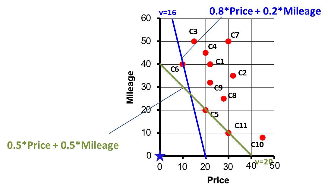
Example: Weighted Preferences and Their Impact
Consider the line of equation , where is a constant representing the score. This can also be written as , from which we can derive that all the lines with the same slope are parallel and represent different scores. By definition, all the pints on the same line are equally good, with higher values indicating less desirable points.
Weights :
Best car: , as it is closest to .
Weights :
Best cars: and , as the weights change the scoring function and shift preferences.
k-Nearest Neighbors (k-NN)
The -NN model evaluates top- queries using distances in a multidimensional attribute space. Instead of ranking by scores, tuples are ranked by their proximity to a target point, using a distance function .
Components of -NN Model:
Attribute Space (): A set of -dimensional ranking attributes , with
Relation (): , where are non-ranking attributes.
Target Point (): Query point , with any
Distance Function (): Measures closeness between tuples and .
Algorithm
Given a point , a relation , an integer , and a distance function , the -NN algorithm retrieves the tuples closest to :
Compute Distances: For each tuple , calculate the distance .
Sort and Select: Sort the tuples in by their distances to and select the top .
Return Results: Output the tuples with the smallest distances.
The most commonly used distance functions are Lp-norms (Minkowski distance).
Relevant cases are:
Euclidean Distance ():
Suitable for circular search areas (hyper-ellipsoids with weights).
Manhattan Distance ():
Ideal for rectangular search areas (hyper-rhomboids with weights).
Chebyshev Distance ():
Useful for box-shaped search areas (hyper-rectangles with weights).
Weights can adjust the importance of dimensions:
Weighted Euclidean Distance:
Weighted Manhattan Distance:
Weighted Chebyshev Distance:
The geometric impact of the weights in distance functions is significant: a larger weight reduces the importance of the corresponding attribute , effectively stretching the search region along that axis. Conversely, a smaller weight increases the importance of , compressing the search region in that direction. This adjustment allows the ranking or nearest neighbor search to reflect user preferences by emphasizing or de-emphasizing specific attributes in the multidimensional space.
Top-k Join Queries
In top- join queries, the goal is to rank results based on combined information from multiple relations.
SELECT <attributes>FROM R_1, R_2, ..., R_nWHERE <join and local conditions>ORDER BY S(p_1, p_2, ..., p_m) [DESC]FETCH FIRST k ROWS ONLY;
Examples
Highest Paid Employee Relative to Department Budget:
SELECT E.*FROM EMP E, DEPT DWHERE E.DNO = D.DNOORDER BY E.Salary / D.Budget DESCFETCH FIRST 1 ROW ONLY;
Two Cheapest Restaurant-Hotel Combos in Italy:
SELECT *FROM RESTAURANTS R, HOTELS HWHERE R.City = H.City AND R.Nation = 'Italy' AND H.Nation = 'Italy'ORDER BY R.Price + H.PriceFETCH FIRST 2 ROWS ONLY;
Top-k 1-1 Join Queries
All joins are based on a common key attribute(s), making this the simplest case to manage and serving as the foundation for more complex scenarios. This approach is practically relevant and involves two main scenarios:
An index is available for retrieving tuples according to each preference.
The relation is distributed across multiple sites, with each site providing information about only a portion of the objects (the “middleware” scenario).
Each input list supports sorted access, where each access returns the ID of the next best object along with its partial (local) score and potentially other attributes. Additionally, each input list supports random access, allowing retrieval of the partial score of an object given its ID (requiring an index on the primary key). The ID of an object remains consistent across all inputs (possibly after reconciliation). Each input contains the same set of objects.
Example
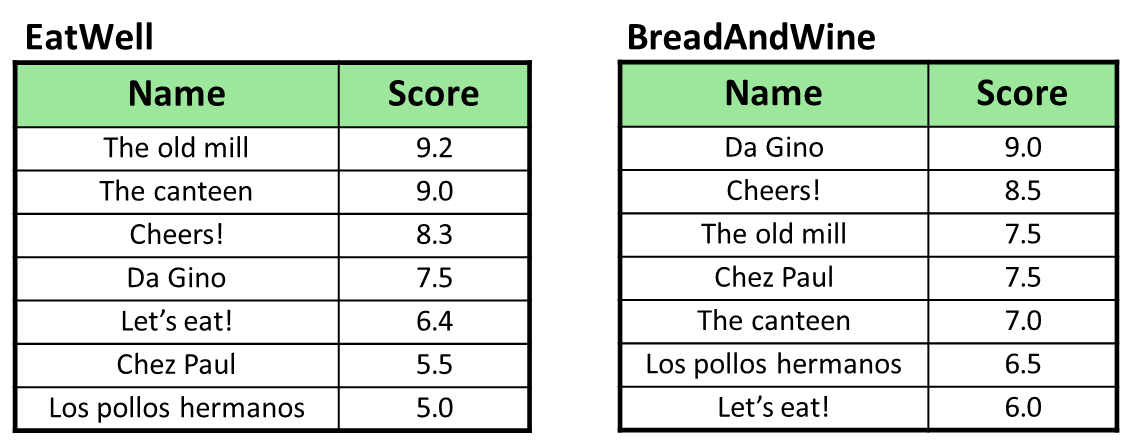
Consider the two tables above that describe the same set of objects but considering the score given only considering how well eating at a restaurant matches the user’s preferences and considering bread and wine preferences, respectively.
The goal is to find the top objects based on a scoring function that combines these local scores.
SELECT *FROM EatWll EW, BreadAndWine BW WHERE EW.Name = BW.NameORDER BY EW.Score + BW.Score DESCFETCH FIRST 1 ROW ONLY;
The resulting table will contain the top objects based on the combined scores from both tables. However, the winner is not the best locally scored object in either table, but rather the one that maximizes the combined score across both tables.
Name
Global Score
Cheers!
16.8
The old mill
16.7
Da Gino
16.5
The canteen
16.0
Chez Paul
13.0
Let’s eat!
12.4
Los pollos hermanos
11.5
A Model for Scoring Functions
Scoring functions are essential to rank objects based on their attributes. Each object has local or partial scores , one for each scoring dimension . These scores are normalized for consistency and mapped to a score space, , where is the number of dimensions.
Definition
The global score combines these local scores into a single value that represents the overall ranking of the object. Formally:
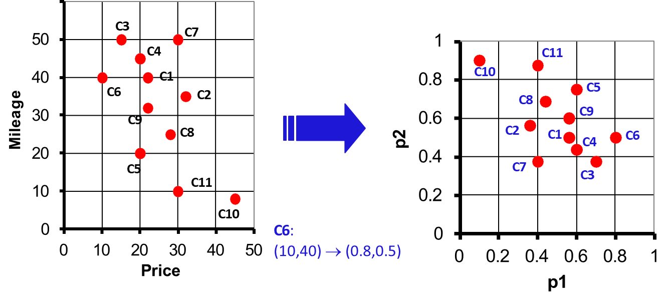
In the score space, objects are represented as points defined by their local scores.
Example
For example, in an attribute space :
Assume:
These transformations map objects into the score space while preserving the relative ranking of scores along each axis.
There are several common scoring functions, each with different properties and implications for ranking:
SUM (or AVG): Assumes equal weight for all attributes.
WSUM (Weighted Sum): Assigns different weights to attributes to reflect their importance.
MIN (Minimum): Ranks objects by their worst local score, ensuring robust evaluation.
MAX (Maximum): Ranks objects by their best local score.
For any scoring function, the goal is to retrieve the objects with the highest global scores. However, efficiency depends on the scoring function used, as some are computationally more demanding.
Definition
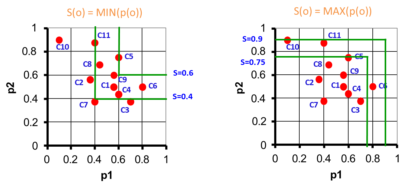
Iso-score curves are sets of points in the score space with the same global score.
Example
For example:
For , iso-score curves are lines in with a slope determined by the weights and .
For , iso-score curves are horizontal and vertical lines intersecting at .
These curves allow visualization of how scoring functions distribute rankings in the score space, analogous to iso-distance curves in geometric spaces.
Efficient Computation of Top-k Results
Challenge
Efficiently compute top- results for a 1-1 join query when the scoring function is complex.
Baseline Algorithm ():
Retrieve the best objects from each input .
Rank these objects by .
Output the top- objects.
Limitation: works well for but may fail for functions like or .
Advanced Algorithms:
Use index structures or dynamic programming for efficient query evaluation.
Leverage sorted access to fetch tuples in ranked order.
Utilize random access to compute scores dynamically for objects retrieved from different relations.
Summary
Algorithm
Function
Data Access
Notes
MAX
Sorted
Instance-optimal
FA
Monotone
Sorted and Random
Cost independent of the scoring function
TA
Monotone
Sorted and Random
Instance-optimal
NRA
Monotone
Sorted
Instance-optimal, but provides approximate scores due to lack of random access
The B0 Algorithm
The algorithm is a foundational method designed to solve top- queries efficiently when the scoring function is defined as . Its simplicity lies in leveraging ranked lists of objects without requiring complex operations such as random accesses or full computation of global scores for all objects. The algorithm is considered instance-optimal, meaning its cost on any input is at most twice the cost of the best algorithm for that input.
Algorithm
The algorithm accepts as input:
An integer , representing the number of top-ranked objects to retrieve.
ranked lists , where each list is sorted by a local scoring criterion.
The output is a set of objects with the highest global scores, computed using the scoring function.
Perform sorted accesses on each of the ranked lists. Store the retrieved objects and their corresponding partial scores in a buffer .
For each object in , calculate its global score as the maximum of its available partial scores.
Return the objects with the highest global scores.
This method avoids retrieving missing partial scores for objects, as it relies solely on the maximum value among the available scores. It also performs no random accesses, making it computationally efficient in scenarios where is the scoring function.
Example
Consider a query with and three ranked lists representing partial scores , , and . The goal is to identify the two objects with the highest global scores
OID
OID
OID
OID
o7
0.7
o2
0.9
o7
1.0
o7
1.0
o3
0.65
o3
0.6
o2
0.8
o2
0.9
o4
0.6
o7
0.4
o4
0.75
o3
0.65
o2
0.5
o4
0.2
o3
0.7
o4
0.6
After performing sorted accesses and computing , the top two objects are and , with scores 1.0 and 0.9, respectively.
While is effective for , it fails for other scoring functions like or .
For instance, consider a case where . If , the algorithm might mistakenly select an object based on partial scores alone, leading to incorrect results.
OID
OID
OID
o7
0.9
o2
0.95
o7
1.0
o3
0.65
o3
0.7
o2
0.8
o2
0.6
o4
0.6
o4
0.75
Performing random accesses to compute yields:
OID
o2
0.6
o7
0.5
However, objects with missing partial scores, such as , might have a global score exceeding the retrieved values, resulting in incorrect results. This issue arises because lacks a mechanism to evaluate lower bounds or complete scores for all objects.
Practical Insights:
Efficiency: The simplicity of makes it computationally efficient for -based queries, avoiding unnecessary accesses and computation.
Scalability: scales well when the number of lists or objects is large, as it processes only a small subset of the data.
Use Case Limitations: For applications requiring other scoring functions, alternative algorithms like TA (Threshold Algorithm) or NRA (No Random Access) must be employed to guarantee correctness and efficiency.
Fagin’s Algorithm (FA)
Fagin’s Algorithm (FA) is a robust approach for computing the top- results from multiple ranked lists, where the scoring function combines these lists through a monotone aggregation function. Unlike algorithms tailored to specific scoring functions, FA operates with a general-purpose stopping condition, making it versatile but less optimized in some cases.
Algorithm
Input: integer , a monotone function combining ranked lists
Output: the top- pairs
Extract the same number of objects by sorted accesses in each list until there are at least objects in common
For each extracted object, compute its overall score by making random accesses wherever needed
Among these, output the objects with the best overall score
The algorithm proceeds in three main phases:
Sorted Access Phase:
Objects are accessed sequentially from each ranked list until at least objects appear in all lists (i.e., common objects are found across the lists). This ensures enough candidates for the final top- computation.
Score Computation Phase:
For each object encountered in the sorted access phase, its global score is computed by making random accesses to retrieve any missing partial scores. These scores are then aggregated using the monotone function .
Selection Phase:
Among all objects with fully computed scores, the objects with the highest global scores are selected as the output.
The algorithm guarantees correctness and is efficient when the scoring function is monotone, as this ensures that objects with higher partial scores in individual lists are favored.
FA is sublinear in the total number of objects , with a complexity of . For example, when combining two lists (), the complexity reduces to . Despite this efficiency, FA is not instance-optimal, meaning there may be scenarios where other algorithms perform better for a given input.
Example: Hotels in Paris
Consider a query to find hotels in Paris with the best combined cheapness and rating. The scoring function is defined as a weighted average:
FA proceeds as follows:
Sorted Access:
Hotels are accessed sequentially from both the cheapness and rating lists.
The process continues until at least hotels appear in both lists.
Cheapness
Score
Rating
Score
Ibis
0.92
Crillon
0.90
Etap
0.91
Novotel
0.90
Novotel
0.85
Sheraton
0.80
Mercure
0.85
Hilton
0.70
Hilton
0.825
Ibis
0.70
Score Computation:
Random accesses retrieve missing scores for overlapping hotels, allowing the computation of their global scores.
For example:
Selection:
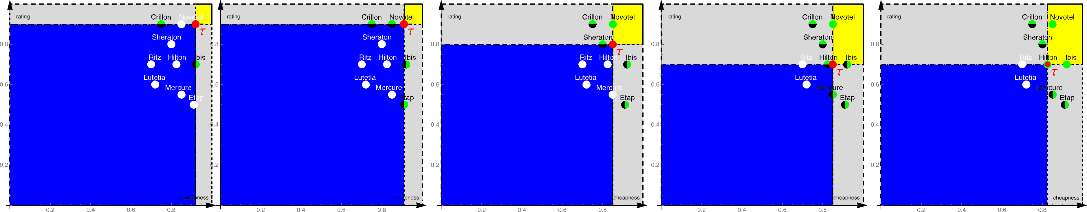
Definition
The threshold point () is defined as the object with the smallest values in all lists during the sorted access phase.
FA stops once the yellow region (fully seen objects) contains at least points. The gray regions represent partially seen objects, while the blue region contains unseen objects that cannot beat the scores in the yellow region.
While FA is versatile, it has several limitations:
Scoring Function Independence:
The algorithm does not exploit specific properties of the scoring function . This generality can result in higher costs compared to specialized algorithms.
Memory Requirements:
FA buffers all objects accessed during the sorted access phase. For large datasets, this can lead to significant memory consumption.
Inefficiency in Random Access:
The sequential nature of sorted access followed by random access can be inefficient. Some improvements, such as interleaving random accesses with score computation, can reduce unnecessary work.
Stopping Condition:
The stopping condition of finding common objects can be suboptimal. Algorithms like TA (Threshold Algorithm) refine this by dynamically updating score bounds.
FA is well-suited for scenarios where:
The scoring function is complex or not explicitly given.
The dataset is relatively small, or memory usage is not a constraint.
General-purpose solutions are preferred over fine-tuned approaches.
Threshold Algorithm (TA)
The Threshold Algorithm (TA) is a powerful and efficient method for computing the top- results from multiple ranked lists. Unlike Fagin’s Algorithm (FA), TA is instance-optimal among all algorithms that utilize both random and sorted accesses. This means that no other algorithm in its class can guarantee better performance on every possible input.
Algorithm
Input: integer , a monotone function combining ranked lists
Output: the top pairs
Do a sorted access in parallel in each list
For each object , do random accesses in the other lists , thus extracting score
Compute overall score . If the value is among the highest seen so far, remember (in a buffer)
Let be the last score seen under sorted access for
Define threshold
If the score of the th object is worse than , go to step 1
Return the current top- objects
TA operates by combining sorted accesses (to retrieve objects sequentially from each ranked list) and random accesses (to gather missing scores of partially seen objects). The algorithm iteratively refines a threshold score to determine when it can safely terminate.
Parallel Sorted Access:
TA begins by sequentially retrieving objects from each ranked list using sorted access.
For each new object encountered in any list, random accesses are made to obtain its scores from other lists , ensuring that its global score can be computed.
Score Computation:
The global score is calculated for each object by aggregating its partial scores using a monotone function .
If ’s score is among the -highest seen so far, it is added to the top- buffer.
Threshold Update:
The threshold is dynamically updated based on the scores of the last objects retrieved via sorted access in each list. The threshold score is given by:
Stopping Condition:
TA terminates when the th highest score in the top- buffer is no worse than the current threshold . At this point, no unseen object can have a score higher than the worst score in the top- buffer.
Final Output: TA returns the objects with the highest scores.
Example: Hotels in Paris with TA
Imagine a query to find the top hotels in Paris based on price and rating, using a scoring function defined as:
Two ranked lists are available, one for cheapness and one for rating:
Hotels
Cheapness
Hotels
Rating
Ibis
0.92
Crillon
0.90
Etap
0.91
Novotel
0.90
Novotel
0.85
Sheraton
0.80
Mercure
0.85
Hilton
0.70
Hilton
0.825
Ibis
0.70
Sheraton
0.80
Ritz
0.70
Crillon
0.75
Lutetia
0.60
Steps of TA:
Perform sorted accesses on both lists:
From the cheapness list:
From the rating list:
Use random accesses to complete missing scores:
Example: For , retrieve cheapness = 0.75 and rating = 0.90. Compute .
Update the threshold:
After accessing the first few hotels, we update the threshold setting it to and the point to .
Stop when the score of the th object in the buffer is no worse than .
Result:
Top 2 Hotels
Score
Novotel
0.875
Crillon
0.825
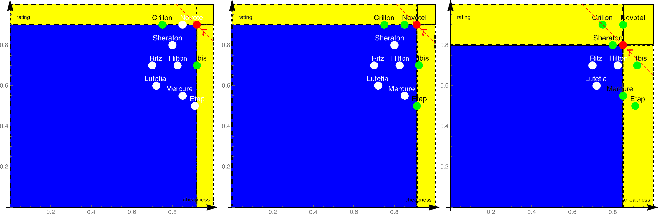
The threshold point represents the lowest possible scores of unseen objects based on the current state of sorted access. By design:
Objects fully seen (yellow region) have accurate scores and can be directly compared.
Partially seen objects (gray region) can only compete if they dominate .
Unseen objects (blue region) cannot have scores exceeding the threshold, ensuring correctness.
The dashed red line separates the region of scores dominating from the rest, reinforcing that no unseen object can outperform the th best seen so far.
TA is highly efficient because it adapts to the specific scoring function and minimizes unnecessary accesses. The cost model for TA is expressed as:
where:
and are the total numbers of sorted and random accesses, respectively.
and are the unit costs for sorted and random accesses.
In many real-world scenarios, random accesses (such as database lookups) are significantly more expensive than sorted accesses (such as index scans), meaning that the cost per random access () is greater than the cost per sorted access (). In some extreme cases, random access may not be possible at all (i.e., ), in which case the Threshold Algorithm (TA) operates using only sorted accesses.
The main advantage of TA is its ability to efficiently compute top- results while minimizing the number of random accesses, making it particularly suitable for applications with large datasets and complex scoring functions.
Instance Optimality: TA is optimal across all instances using both access types, unlike FA, which does not leverage scoring function properties.
Scoring Function Adaptation: TA dynamically adjusts its operations based on the monotone function , ensuring efficient processing.
Lower Middleware Costs: By reducing unnecessary accesses, TA often outperforms FA in practical applications.
TA is ideal for applications where:
Random access costs are not prohibitively high.
The scoring function is monotone and well-defined.
Efficient use of resources (e.g., memory, access time) is crucial.
The No Random Access (NRA) Algorithm
The NRA (No Random Access) algorithm is designed for scenarios where random access to data is not feasible or practical.
Its primary goal is to identify the top- objects from a set of ranked lists while keeping the cost of computation as low as possible.
Unlike algorithms that rely on precise scores for ranking, NRA acknowledges uncertainty and computes bounds for scores to approximate the top- results.
Key concepts of NRA:
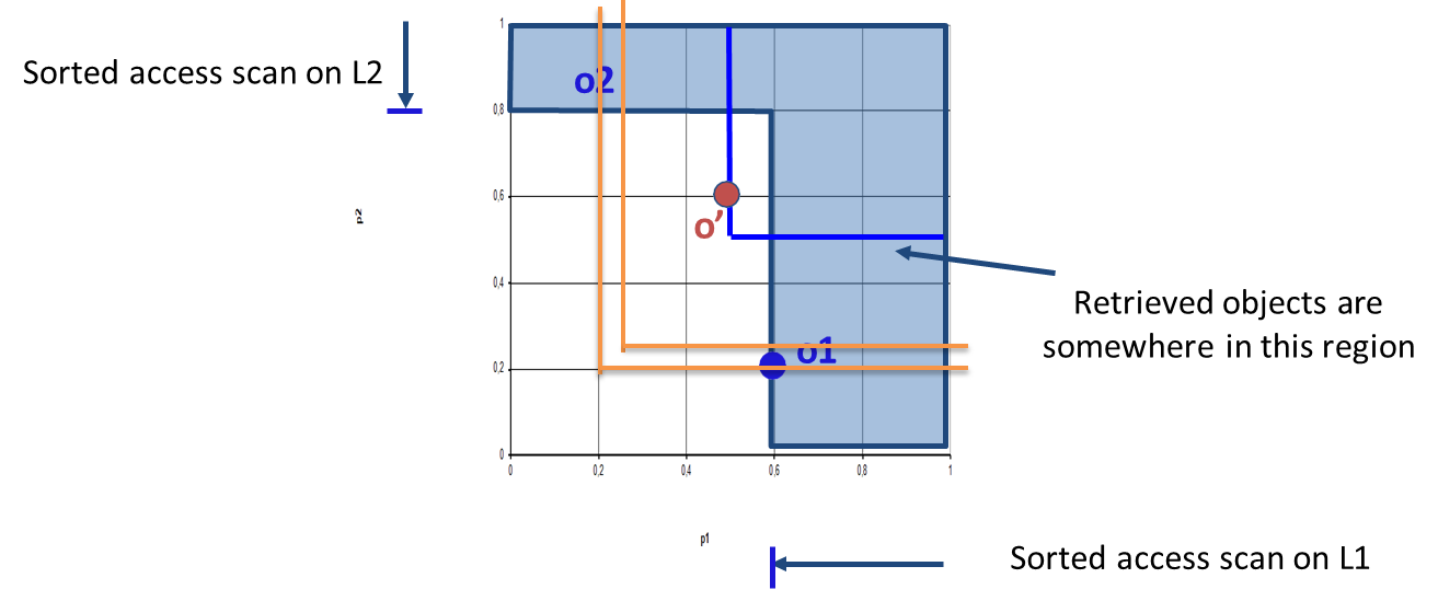
Score Bounds:
For each object retrieved via sorted access, the algorithm maintains:
A lower bound, , which represents the minimum possible score of based on the data retrieved so far.
An upper bound, , which represents the maximum possible score of .
Buffer Management:
The algorithm employs a buffer with unlimited capacity to store objects retrieved during sorted access. This buffer is kept sorted in descending order of the objects’ lower bound scores, .
Threshold Point:
A threshold is maintained to represent the upper bound of scores for unseen objects. This threshold provides an additional constraint for evaluating whether further iterations are necessary.
Termination Condition:
By maintaining a set of the current best objects, the algorithm halts when it becomes clear that no object not in can outperform any of the objects within it. So
i.e, when beats both the max value of among the objects in and the score of the threshold point .
Algorithm
Input: integer , a monotone function combining ranked lists
Output: the top- objects according to
Initialize:
Begin with an empty buffer and make a sorted access to each of the ranked lists .
Update Buffer:
For each object retrieved, calculate its lower bound and upper bound . Store in , ensuring it remains sorted by .
Iterative Refinement:
Repeat the process of accessing lists and updating until the termination condition is met. This ensures the algorithm identifies the top- objects.
Output:
Return the set of objects in with the highest lower bound scores.
The computational cost of the NRA algorithm does not always increase with larger values of. In certain cases, identifying the top- objects can require less work than finding the top-, due to the way score bounds are refined and objects are eliminated from consideration.
NRA is instance-optimal among algorithms that rely solely on sorted access and avoid random access. For any given input, it guarantees the best possible performance within its class, with an optimality ratio equal to , the number of ranked lists being combined.
A distinctive aspect of NRA is its handling of uncertain scores. Since random access is not used, the algorithm may only be able to provide approximate scores for some objects in the final result, reflecting the uncertainty inherent in the available data.
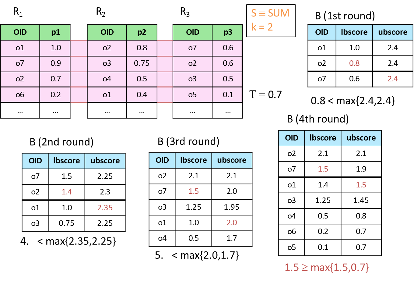
Example of NRA in Action
Consider a scenario with three objects , , and , and the following details:
:
The algorithm identifies as the top object with a score . NRA requires accessing all but the last rank of the lists to confirm this result.
:
To determine the top-2 objects ( and ), only three rounds of access are necessary, as quickly emerges as the second-best option.
Skyline Queries
Skyline queries are a powerful tool in multi-criteria decision-making, often used to identify the best options among a dataset according to multiple perspectives. They rely on the concept of dominance, which is central to their operation.
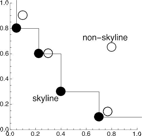
Intuitively, a tuple in a dataset is said to dominate another if it is equal or better across all dimensions and strictly better in at least one dimension. In practical terms, lower values are typically preferred (e.g., lower price or distance).
The result of a skyline query is the set of non-dominated tuples, representing the most desirable options under various criteria.
Definition
Mathematically, a tuple dominates another tuple , denoted , if and only if:
For every dimension (): (i.e., is nowhere worse than ).
For at least one dimension (): (i.e., is strictly better in at least one aspect).
The set of all non-dominated tuples is called the skyline of the relation. This concept is also known as the Pareto-optimal set in multi-objective optimization or the maximal vectors problem in computational geometry. Graphically, in two dimensions, the skyline can resemble the contour of the dataset when visualized.
Skyline queries differ from top- queries in that they do not rely on a single scoring function. Instead, they identify all potentially optimal tuples, regardless of any specific weighting of attributes. This flexibility makes them particularly useful when user preferences are not explicitly defined or when exploring trade-offs among attributes.
SQL Representation of Skyline Queries
Skyline queries are not part of the SQL standard, but proposed syntaxes have been developed for their implementation. A possible syntax might look like this:
SELECT ... FROM ... WHERE ... GROUP BY ... HAVING ...
SKYLINE OF [DISTINCT]   d1 [MIN | MAX | DIFF], ...,
						dm [MIN | MAX | DIFF]
ORDER BY ...
and a possible example of a skyline query could be:
SELECT * FROM Hotels WHERE city = 'Paris'SKYLINE OF price MIN, distance MIN
This query identifies hotels in Paris that are optimal based on the minimal price and distance criteria. Internally, this can be translated into standard SQL using subqueries and dominance conditions:
SELECT * FROM Hotels h WHERE h.city = 'Paris' AND NOT EXISTS ( SELECT * FROM Hotels h1 WHERE h1.city = h.city AND h1.distance <= h.distance AND h1.price <= h.price AND (h1.distance < h.distance OR h1.price < h.price))
This translation explicitly checks for dominance by ensuring that no other tuple dominates the current one.
Algorithms for Computing Skylines
Skyline queries can be computed using different algorithms, each with distinct trade-offs in terms of efficiency and practicality.
The Block Nested Loop (BNL) algorithm is simple and intuitive, iteratively comparing each point to those already identified as potential skyline candidates. However, its quadratic time complexity () makes it unsuitable for large datasets.
In contrast, the Sort-Filter-Skyline (SFS) algorithm first sorts the data using a monotone function, which allows skyline points to be identified more efficiently during a single pass. This reduces the computational complexity to , making SFS preferable for larger datasets.
While BNL is easier to implement and requires no pre-processing, SFS offers significant performance improvements by leveraging sorting and early elimination of dominated points.
Algorithm
Approach
Strengths
Limitations
Complexity
BNL
Compare each point to current skyline set
Simple, no pre-processing
Slow for large datasets
SFS
Sort, then filter for skyline points
Efficient for large data
Requires sorting upfront
Block Nested Loop (BNL)
The Block Nested Loop (BNL) algorithm is a straightforward approach to computing skylines.
Algorithm
Input: a dataset of multi-dimensional points
Output: the skyline of
Initialize the skyline set as an empty set.
For every point in , if the point is not dominated by any point in , then:
Remove from the points dominated by .
Add the point to the set .
Return the skyline set .
While conceptually simple, BNL has a computational complexity of , where is the number of points in the dataset. This makes it inefficient for large datasets.
Sort-Filter-Skyline (SFS)
The Sort-Filter-Skyline (SFS) algorithm improves upon BNL by leveraging pre-sorting. By sorting the dataset according to a monotone function of its attributes, SFS ensures that no later tuple can dominate an earlier one.
Algorithm
Input: a dataset of multi-dimensional points
Output: the skyline of
Sorting Phase: The dataset is sorted based on a monotone function, such as the sum of all attribute values. This ensures that points are processed in an order that facilitates skyline identification.
Initialize a skyline set as an empty set.
For every point in the sorted dataset , if is not dominated by any point in , then add that point to the skyline set .
Return the skyline set .
Pre-sorting reduces unnecessary comparisons and allows immediate identification of skyline points during iteration. The computational complexity is reduced to , making it more practical for larger datasets.
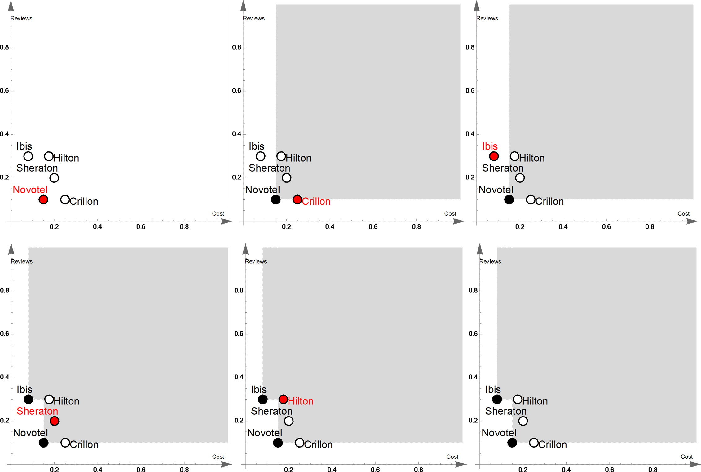
Example
Consider again the example of hotels in Paris. Using SFS, we can efficiently compute the skyline by first sorting the hotels based on their price and their complaints.
Hotel
Price
Complaints
Ibis
0.8
0.3
Novotel
0.15
0.1
Hilton
0.175
0.3
Crillon
0.25
0.1
Sheraton
0.2
0.2
The sorted list based on the sum of price and complaints would look like this:
Hotel
Price ⬆️
Complaints
Novotel
0.15
0.1
Crillon
0.25
0.1
Ibis
0.8
0.3
Sheraton
0.2
0.2
Hilton
0.175
0.3
Then, we add if not dominated by any point in and remove dominated points, leading to the final skyline set. The final window of skyline points would include Novotel and Ibis, as they are not dominated by any other hotel in terms of both price and complaints.
Hotel
Price
Complaints
Novotel
0.15
0.1
Ibis
0.8
0.3
Strengths and Limitations of Skyline Queries
Skyline queries are highly effective for identifying potentially interesting objects when user preferences are unknown or undefined. They provide a comprehensive overview of all non-dominated options, requiring no parameters or pre-specified scoring functions. However, this agnostic approach comes with limitations.
For large datasets, particularly those with anti-correlated attributes, the number of skyline points can become excessively large, making the results difficult to interpret. Additionally, the computational cost remains high for quadratic algorithms like BNL. While SFS mitigates this to some extent, it may still struggle with extremely large datasets or complex dominance relationships.
The k-Skyband
To address the issue of excessive result sizes, the concept of -skybands has been introduced. A -skyband includes all tuples that are dominated by fewer than other tuples. This allows for finer control over the size of the result set. For example:
The skyline is equivalent to the 1-skyband.
A top- result set is always contained within the -skyband.
By adjusting , users can balance the comprehensiveness of the results with their cardinality.
Comparing Skyline Queries to Ranking Queries
Skyline queries and ranking queries serve different purposes and are suited to different scenarios. While skyline queries provide a broad overview of all potentially optimal options, ranking queries focus on identifying a small, prioritized subset based on a specific scoring function.
Aspect
Ranking Queries
Skyline Queries
Simplicity
Moderate complexity
Very simple
Overview of interesting results
Limited
Comprehensive
Control of result size
Yes
No
Trade-offs among attributes
Explicit control
Implicit (dominance)
Ranking queries are ideal when user preferences are well-defined and a limited result set is desired. Skyline queries excel in exploratory analysis, where trade-offs among attributes need to be understood without committing to a specific scoring function.