System Identification
System identification is a discipline that focuses on the development of mathematical models to describe and analyze various phenomena or systems. The objective of this field is to establish a precise and structured representation of how inputs, which act as causes, influence outputs, which are the resulting effects. By formulating mathematical models, it becomes possible to understand, predict, and control the behavior of a system based on observed data.
A system (
A model (
 Several types of systems can be analyzed using system identification methods. In economic systems, a typical example is the relationship between education levels and income. Economic theories suggest that higher educational attainment generally leads to increased earning potential, but this relationship is influenced by multiple factors such as labor market demand and economic policies. In the social domain, an important system to analyze is the correlation between crime rates and unemployment. Empirical studies often indicate that higher unemployment can lead to increased crime rates due to economic stress and lack of social stability, though other sociopolitical variables also contribute to this dynamic. In the field of physics, a fundamental example is the relationship between electric current and voltage in an electrical circuit. This relationship is governed by Ohm’s law, which states that the current flowing through a conductor is directly proportional to the voltage applied and inversely proportional to the resistance of the conductor.
System identification methods are essential for building predictive models and optimizing real-world systems. By collecting data, applying statistical techniques, and refining mathematical models, researchers and engineers can enhance system performance, make informed decisions, and develop control strategies tailored to specific applications.
Three Approaches to Modeling
In system identification, modeling approaches can be classified into three main categories: white-box modeling, black-box modeling, and gray-box modeling. These approaches differ in the extent to which prior knowledge about the system is incorporated into the model and the methodology used to determine the system parameters. The choice of approach depends on factors such as the availability of physical laws, experimental data, computational resources, and the complexity of the system.
White-Box Modeling
White-box modeling is based entirely on physical laws and prior knowledge about the system. This approach assumes that all aspects of the system are well understood and can be described using fundamental principles, such as Newtonian mechanics, thermodynamics, or electrical circuit theory.
For example, consider a mechanical damper described by the second-order differential equation:
Since all parameters (
| Advantages | Disadvantages | |
|---|---|---|
| The model provides a clear physical interpretation of the system variables. | It requires complete prior knowledge of the system, which is often unrealistic. | |
| It can be generalized to similar systems without requiring new data collection. | Model development is time-consuming and computationally expensive. | |
| It is not feasible for complex systems, where certain interactions may be unknown or difficult to model precisely. |
Black-Box Modeling
Black-box modeling, in contrast, relies entirely on experimental data rather than prior knowledge of the system’s internal mechanisms. The model is built by fitting a mathematical function to observed input-output relationships, often using statistical or machine learning techniques.
For example, in the case of a discrete-time system, a typical black-box representation is given by the transfer function:
where the coefficients
| Advantages | Disadvantages | |
|---|---|---|
| Can be implemented even without deep knowledge of the process. | Lacks physical interpretability, making it difficult to understand the underlying mechanisms of the system. | |
| Fast and cost-effective since it relies on data collection rather than theoretical derivation. | Not generalizable: If the system changes, a new set of experiments must be conducted to update the model. |
Gray-Box Modeling
Gray-box modeling is a hybrid approach that combines the strengths of both white-box and black-box modeling. It assumes that the general form of the system equations is known based on physical principles, but some parameters remain unknown and must be estimated from data.
For example, in a mechanical system, the governing equations may be known, but the damping coefficient or stiffness might need to be inferred from experimental data. The model is then refined using parameter estimation techniques, such as least squares or Bayesian inference.
| Advantages | Disadvantages | |
|---|---|---|
| Retains physical interpretability, as the model structure is based on first principles. | Requires some prior knowledge of the system, making it unsuitable when no theoretical background is available. | |
| Faster to develop than white-box models since not all parameters need to be predetermined. |
Model Assessment
Once a model is developed, it is crucial to assess its accuracy in representing the real system. The modeling error is a measure of the discrepancy between the actual system output and the model’s simulated output.
 Given a system
where
To quantify model accuracy, several evaluation metrics can be used, including:
- Mean Squared Error (MSE): Measures the average squared deviation between observed and predicted values.
- Coefficient of Determination (
): Indicates how well the model explains the variability in the data. - Mean Absolute Error (MAE): Computes the average magnitude of errors without considering their direction.
A well-validated model should not only minimize error but also generalize well to unseen data, ensuring robustness and reliability in practical applications.

Static Systems
A static system is a system in which the output at any given instant depends solely on the input at the same instant. In other words, the system has no memory or dependency on past inputs; knowing the current value of the input variables is sufficient to determine the output.
A classical example of a static system is an electrical resistor, where the relationship between the input voltage
In the field of machine learning, static systems are commonly modeled using black-box approaches, where the goal is to learn an input-output relationship purely from data. One key example of this is regression analysis, where a function is estimated to map input features to continuous outputs.
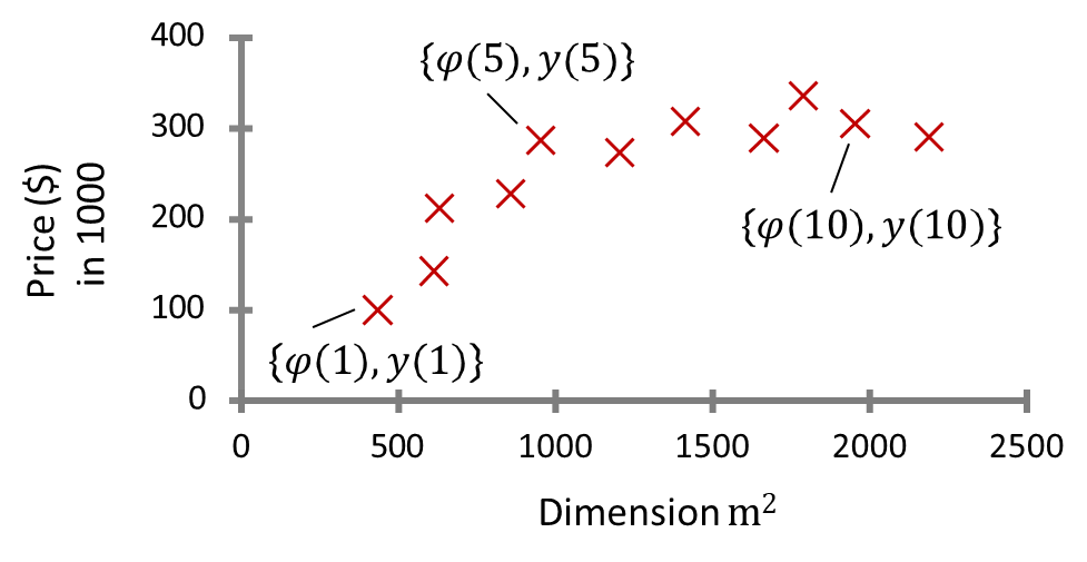
Example: House Price Estimation
Consider the task of predicting the price of a house based on its size. In this case, we define:
- Input (Feature):
= house area in square meters. - Output:
= house price in thousands of dollars. Mathematically, we seek a function
such that: where
is an unknown function that must be learned from data. The following dataset provides some real estate values in the Boston area:
Area (m²) Price (1000$) 523 115 645 150 708 210 1034 280 2290 355 2545 440 Since the output variable
is a continuous value, this problem falls into the category of regression, a fundamental task in supervised learning. The goal is to estimate a function that best fits the given data points. A common approach is to assume a linear model of the form:
where
(intercept) and (slope) are the parameters to be determined using techniques such as least squares regression or gradient descent. In more complex cases, non-linear models such as polynomial regression, support vector regression (SVR), or neural networks may be used to capture intricate relationships between house size and price.
Static systems play a crucial role in many real-world applications where outputs depend only on current inputs. In machine learning, black-box modeling of static systems is a common practice, particularly in regression tasks where the goal is to learn functional relationships between input features and continuous outputs. By leveraging data-driven techniques, we can build predictive models capable of generalizing to unseen cases, making them valuable tools in various domains such as real estate pricing, finance, and industrial applications.
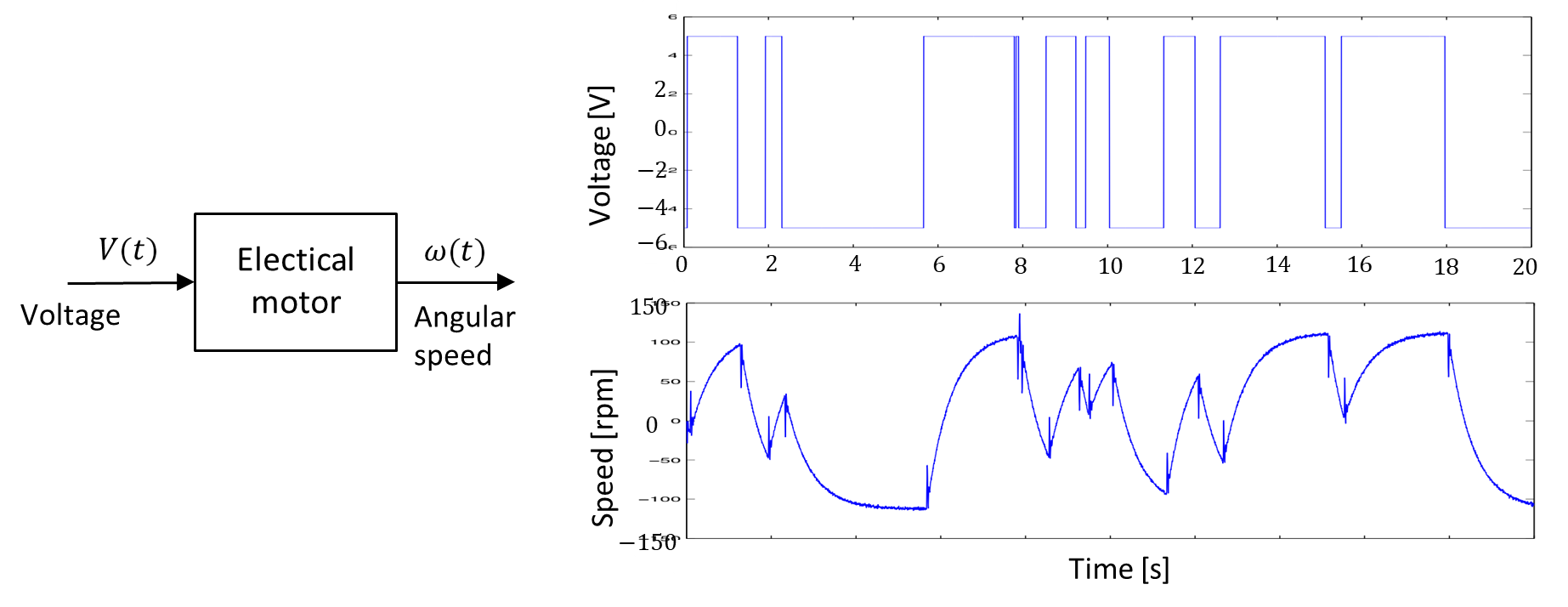
Dynamical Systems
A dynamical system is a system characterized by its ability to “remember” past behaviors, meaning that the current state of the system is influenced not only by the present input but also by its historical behavior. This concept introduces a time-dependent element where the output does not simply respond to the current input but evolves over time, making the time dimension crucial.
In contrast to static systems, where the output is determined by the current input, dynamical systems exhibit memory, meaning the past states of the system play an essential role in determining future behavior. This “memory” aspect is intrinsic to many natural and physical phenomena, such as the evolution of audio signals, hormone concentration in the body, pollutant levels in the environment, and many others.
Examples of Dynamical Systems
- Audio signals: The sound you hear before and after transmission. The quality of the output depends on both the original input and the way the signal evolves during transmission.
- Torque in engines: The current torque can depend on previous values of torque and other system inputs.
- Medicine: The concentration of a medicine in the bloodstream over time, where current concentrations depend on past dosages and metabolic processes.
- Rainfall: The amount of rainfall over time can influence soil moisture and hydrological behavior, which then affects future rainfall.
- Pollutant concentration: The concentration of pollutants in the air or water depends not only on current emissions but also on the cumulative effect of previous emissions and environmental factors.
The description of a dynamical system can be done either in continuous time or discrete time. In continuous-time systems, the evolution of the system is described by ordinary differential equations (ODEs), which capture how a variable changes over an infinitesimally small time interval. An example of such a system is the following ODE:
The derivative,
However, in practical applications, especially in digital computing, we can only handle discrete amounts of data. Therefore, signals must be sampled at regular time intervals,
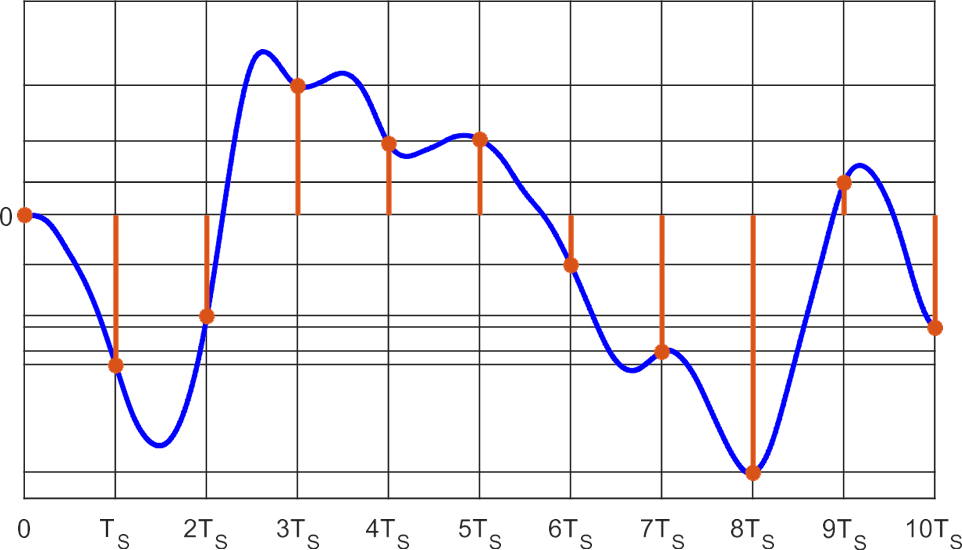
In this course, we will focus on discrete-time systems, where the evolution of the output is described by difference equations rather than differential equations. For example:
In this equation,
In dynamical systems, we still aim to learn a function
where
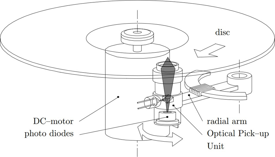
Example: Control of the CD Player
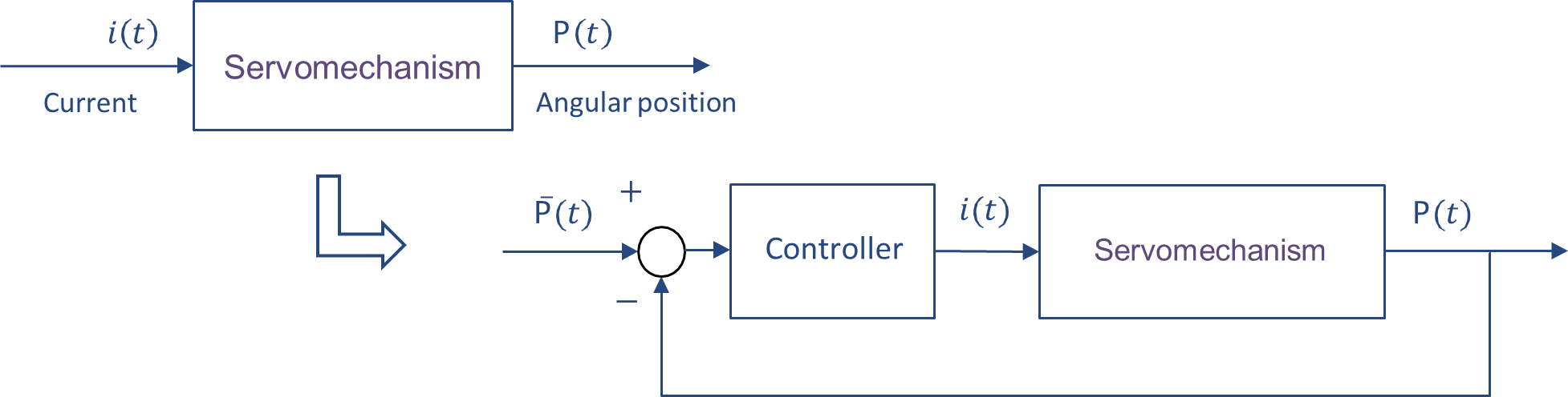
The objective of this example is to position the laser head of a CD player onto the correct track using a mechanical arm. The system we are concerned with involves controlling the current
supplied to the motor that drives the radial arm. This motor moves the arm, which positions the laser source. The position of the laser beam is then measured through photodiodes.
The goal is to design a controller that ensures the laser head is positioned accurately, and that the system has a control bandwidth of 1000 Hz (with the model being valid up to 10,000 Hz).
First Trial: White-Box Model
To model this system, we start with a white-box model, which is based on known physical principles. The key relationship in this model is between the current
supplied to the motor and the torque generated by the motor, which drives the mechanical arm. The relationship is given by the torque equation for a DC motor, where the torque is proportional to the current: Here,
is the motor constant, and the torque is related to the motor’s mechanical dynamics. Assuming no friction and applying Newton’s law of motion to the motor and arm system, we have: where:
is the inertia of the motor and arm system, is the acceleration of the laser head (second derivative of position ). This equation describes the system as a double integrator. The position of the laser head
is obtained by integrating the torque twice, reflecting the motor’s dynamics in a mechanical system. To understand the system in the frequency domain, we apply the Laplace transform. Taking the Laplace transform of the equation, we obtain the transfer function: where
is the Laplace transform variable (complex frequency), and represents the system’s transfer function. This equation reveals that the system behaves as a second-order integrator. Based on this white-box model, a controller can be designed to regulate the position of the laser head by adjusting the current to the motor. However, the controller designed using this model fails to meet the desired bandwidth of 1000 Hz, and undesired vibrations are observed in the system.
This failure indicates that the high-frequency modes of the system, which are not captured by the simple white-box model, are crucial in achieving the desired performance. These modes may arise from factors like friction, structural dynamics, and electromagnetic effects in the motor, which are not accounted for in the basic physical model of the system.
Comparison Between White-Box and Black-Box Models
While the white-box model provides a basic understanding of the system’s behavior, it overlooks higher-frequency dynamics and non-ideal effects. To address these limitations, a black-box model would be necessary. The black-box model would be data-driven, relying on experimental measurements of the system’s behavior (such as input-output data) to estimate the system’s response without making assumptions about the underlying physical laws.
The advantage of the black-box model is that it can capture the high-frequency modes that are crucial for the controller design, as these modes are often too complex or subtle to be modeled accurately using only physical laws. This allows the controller to be designed more accurately for the full range of frequencies, including those beyond the simple dynamics predicted by the white-box model.
In summary, while the white-box model offers an initial understanding of the system’s behavior, it falls short in capturing high-frequency dynamics necessary for an accurate controller design. The black-box approach can address these limitations by modeling the system’s behavior more comprehensively, ensuring that the system meets the required bandwidth and performance criteria.
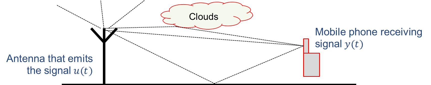
Example: Signal Reception in Mobile Telephony
In mobile telephony, the signal
that is received by the mobile device is a delayed version of the signal that was emitted by the transmitter. This delayed version is a sum of various copies of , each shifted by a different amount of time. The received signal can be modeled as: where
are the gain factors for each delayed version of the signal, are the corresponding delays, and represents noise. The goal is to reconstruct the transmitted signal from the received signal . In general, the received signal can be written in a more compact form as: where
is the channel model that describes how the signal is affected by the transmission medium (e.g., mobile network), and is the noise introduced by the channel. Here, is a time-shift operator that describes the relationship between the transmitted and received signals. The task at hand is to reconstruct the transmitted signal
based on the received signal . If the model were known, and the data were noiseless, the transmitted signal could be obtained by: However, the channel model
is unknown because it depends on factors like the position of the mobile phone, which can vary over time as the phone moves. Additionally, the received signal is contaminated by noise , which makes the reconstruction more challenging. The challenge arises from the fact that
is unknown and it changes dynamically with the position of the mobile phone. Since the phone is mobile by definition, the channel conditions (such as the distance from the base station and obstacles between the transmitter and receiver) vary as the phone moves, causing fluctuations in the signal quality. Thus,
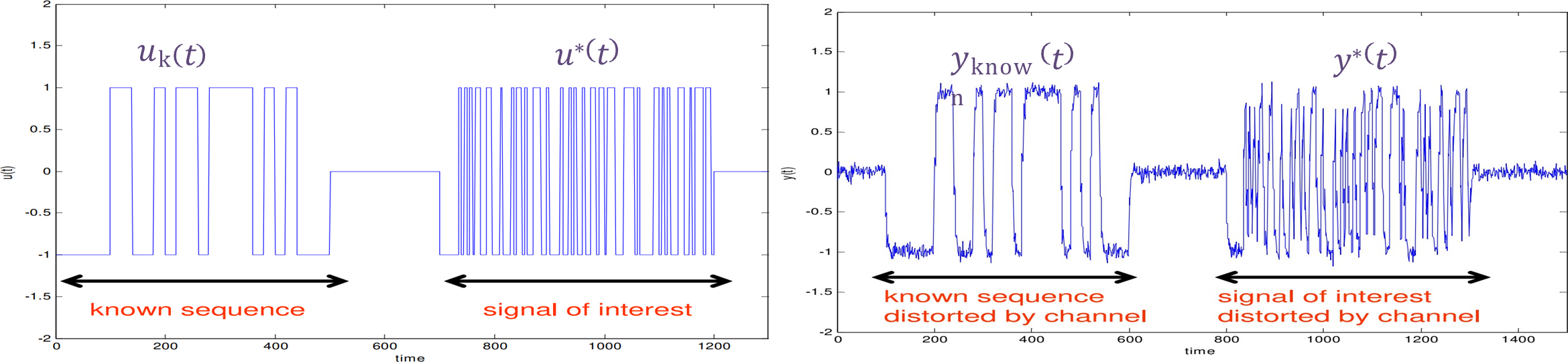
cannot be directly inferred from the received signal without additional information. o address this problem, a model identification technique is employed. When a mobile phone is engaged in a call, the GSM software uses a known reference signal to estimate the channel model
. The key idea is that the signal of interest, denoted , is preceded by a known signal , which is transmitted at the start of the communication. Both (the signal of interest) and (the known signal) are affected by the transmission channel, but since is known, it can be used to identify the channel model.
The GSM system can use this reference signal
along with the received signal to estimate the dynamical model of the channel . Once the model is estimated, the signal of interest can be recovered by applying the inverse of the estimated channel model: Here,
is the received signal that contains the signal of interest along with the effects of the transmission channel and noise. The inverse of is applied to filter out the channel effects, thereby reconstructing the transmitted signal . In mobile telephony, the process of signal reception is affected by delays and distortions introduced by the transmission channel. To reconstruct the transmitted signal
, the channel model needs to be identified. By using a known reference signal and the received signal , the GSM software estimates the channel model and subsequently applies this model to recover the original transmitted signal. This approach ensures that even with noisy and distorted signals, the transmitted information can be accurately reconstructed.