Performance Bound

Performance bounds provide valuable insight into the primary factors affecting the performance of computer systems. They can be computed quickly and easily, therefore serving as a first-cut modeling technique. Several alternatives can be treated together. We will consider single-class systems only and determine asymptotic bounds, i.e., upper and lower bounds on a system’s performance indices (throughput) and (response time). In our case, we will treat and bounds as functions of the number of users/arrival rate (i.e., ).

The advantages of bounding analysis are that they highlight and quantify the critical influence of the system bottleneck. The can be computed quickly, even by hand, and are useful in system sizing based on preliminary estimates. This kind of studies typically involve a large number of candidate configurations with a single critical resource (e.g., CPU) dominant and the other configured accordingly, treated as one alternative. They are also useful for system upgrades.

Bottleneck

Definition

The bottleneck is the resource within a system that has the greatest service demand. Its service demand is , denoted .

The bottleneck resource is important, because it limits the possible performance of the system. This will be the resource that has the highest utilization in the system.

Notation

The considered models and the bounding analysis make use of the following parameters:

• , the number of service centers
• , the sum of the service demands at the centers, so
• , the largest service demand at any single center
• , the average think time, which represents the time spent by a user thinking or performing other non-computational tasks while waiting for a response in interactive systems

These parameters are important in determining the performance of computer systems. The performance quantities that are considered in the analysis are:

• , the system throughput, which represents the number of jobs completed per unit of time
• , the system response time, which represents the time taken for a job to complete from the moment it enters the system until it receives a response

By analyzing these parameters and performance quantities, we can derive bounds on the system’s performance under different conditions, such as light load and heavy load. These bounds provide valuable insights into the system’s behavior and help in system sizing and performance estimation.

Asymptotic bounds

The bounding analysis is based on the assumption that the service demand of a customer at a center does not depend on how many other customers currently are in the system or at which service centers they are located. This allows us to derive asymptotic bounds that provide upper and lower limits on the system's performance indices and .

Asymptotic bounds are derived by considering the (asymptotically) extreme conditions of light and heavy loads. We can derive both optimistic and pessimistic bounds on the system’s performance indices and under these conditions.

• Optimistic: upper bound and lower bound. The optimistic bounds correspond to the best-case scenario, where the system performs at its maximum capacity
• Pessimistic: lower bound and upper bound. The pessimistic bounds correspond to the worst-case scenario, where the system is overloaded and performance is severely degraded

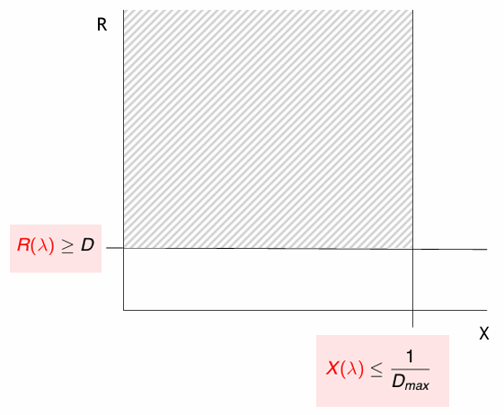
Open models

The bound is the maximum arrival rate that the system can process. We define as the arrival rate, and as the throughput, so . If bound, the system saturates, and new jobs have to wait an indefinitely long time. The utilization of a resource, denoted as , is equal to , so

The bound is calculated as:

The bounds are the largest and smallest possible experienced at a given , and are investigated only when (otherwise the system is unstable). The two extreme situations are:

• If no customers interfere with any other, then , with
• If customers arrive together every time units, there is no pessimistic bound on . Customers at the end of the batch are forced to queue for customers at the front of the batch, and thus experience large response times. The batch can be extremely long, , and there is no pessimistic bound on response times, regardless of how small the arrival rate might be.

Bound for	Bound for

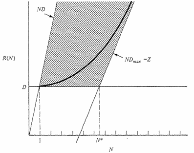
Closed models

The bounds are considered first, then converted in bounds using Little’s Law.

bounds

Light Load situation (lower bounds): in the light load situation, the system is not saturated, and the smallest possible is obtained with the largest , i.e., new jobs queue behind others already in the system. In the case of only one customer, we have (following the response time law):

Then is:

Adding customers, the smallest is obtained with the largest , i.e., new jobs queue behind others already in the system. In closed models, the highest possible system response time occurs when each job, at each station, finds all the other customers in front of it, so . In this case, and is:

Largest is obtained with the lowest response time , which means no conflicts. The lowest response time can be achieved if a job always finds the queue empty and starts being served immediately. If new jobs never queue behind others already in the system, then , and is:

Heavy Load situation (upper bound): in the heavy load situation, the system is saturated, and the largest possible is obtained with the smallest , i.e., new jobs are served immediately. The utilization of a resource, denoted as , is:

Since the first to saturate is the bottleneck,

Formulas

So, the bounds are

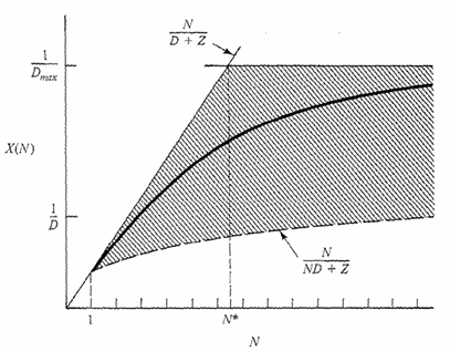
We can define a particular population size determining if the light or the heavy load optimistic bound is to be applied.

bounds

Let us simply rewrite the previous equation, considering that , we have:

and to have as numerator we invert the members and we have

Formula

The bounds are

Bound for	Bound for