To understand instruction scheduling in statically scheduled processors, it is essential to grasp the underlying goal: to reorder instructions in the object code in a way that preserves the original program semantics while minimizing total execution time. In this context, instructions are arranged such that time-critical operations are executed efficiently, and the number of independent instructions that can be issued in parallel is maximized. The more parallelism we exploit, the fewer the clock cycles required to complete a basic block.
The foundation of instruction scheduling lies in the concept of a basic block.
Definition
A basic block is a straight-line sequence of code instructions with only one entry point—no instruction within the block is the target of a jump or branch from outside. It also has only one exit point, typically the last instruction, which may transfer control elsewhere (e.g., a conditional branch, function call, or return).
Since control flow within a basic block is linear and predictable, compilers can more easily apply scheduling optimizations without worrying about unpredictable jumps.
To analyze and optimize the execution of a basic block, we first need to understand the dependencies between instructions. The most common formalism for this is the dependence graph, also known as a Directed Acyclic Graph (DAG). Each node in the graph corresponds to an instruction, and directed edges indicate data dependencies between instructions.
Example
For instance, consider the following sequence:
A = B + 1X = A + CA = E + C
This sequence has several overlapping dependencies. The first instruction writes to A, which is read by the second instruction—this is a Read After Write (RAW) dependency. The third instruction also writes to A, which leads to a Write After Write (WAW) conflict with the first instruction, and a Write After Read (WAR) conflict with the second instruction.
The corresponding dependence graph visually captures these constraints:
graph LR
    1[A = B + 1]
    2[X = A + C]
    3[A = E + C]

    1 -- RAW A --> 2
    1 -. WAW A .-> 3
    2 -. WAR A .-> 3
In scheduling, the goal is to respect these dependencies while fitting instructions into clock cycles in a way that reduces idle functional units and avoids hazards.
To identify bottlenecks and performance limits, we analyze the critical path within the dependence graph. Each node in the graph is annotated with its latency, representing the number of cycles it takes to execute. The longest path through the graph, considering these latencies, defines the minimum theoretical execution time for the basic block—this is known as the Longest Critical Path (LCP).
Formula
Mathematically, for a node i:
For example, consider a more complex basic block involving multiple operations such as multiplications, additions, and stores:
graph LR
    a((a * : 3/3))
    b((b + : 1/1))
    c((c + : 1/1))
    d((d * : 6/3))
    e((e - : 2/1))
    f((f st : 4/2))
    g((g - : 7/1))

    a --> d --> g
    b --> e --> f --> g
    c --> f
In this graph, the numbers beside each node represent the operation’s priority and its latency. The critical path—here represented by the longest data-dependent chain a --> d --> g—determines the minimum number of cycles required to complete execution, assuming an unlimited number of functional units.
The Scheduling Problem
The core challenge of instruction scheduling is to assign a start cycle to each instruction, such that all dependencies are respected, and operations do not conflict in resource usage. In resource-unconstrained scheduling (e.g., ideal ALUs, multipliers, and memory ports), the goal is simply to minimize total execution time.
A fundamental tool for this is the Ready List, which contains operations that are ready to be issued because all their predecessors have been scheduled and their operands are available. From this, scheduling algorithms can determine how to assign instructions to cycles.
Comparison of ASAP and List-Based Scheduling Algorithms
Feature
ASAP Scheduling
List-Based Scheduling
Objective
Minimize start time of each instruction without considering resource constraints.
Minimize execution time while respecting resource constraints.
Considers resource availability and functional unit constraints.
Dependency Handling
Respects data dependencies only.
Respects both data dependencies and resource conflicts.
Instruction Priority
No explicit priority; schedules as soon as dependencies are resolved.
Prioritizes instructions based on critical path or heuristics.
Ready List
Contains all instructions whose dependencies are resolved.
Contains instructions ready for execution, filtered by resource availability.
Use Case
Ideal for generating a baseline schedule or in resource-unconstrained environments.
Suitable for real-world scenarios with limited hardware resources.
Complexity
Simpler to implement.
More complex due to resource management and priority handling.
Output Schedule
May result in resource conflicts or idle cycles.
Produces a more efficient schedule by balancing resource usage.
Example Application
Early-stage scheduling in compilers.
Final-stage scheduling in compilers for VLIW or superscalar architectures.
The ASAP (As Soon As Possible) Scheduling Algorithm
One of the simplest and most commonly used scheduling algorithms is ASAP scheduling.
The idea is to place each instruction in the earliest possible cycle, constrained only by the readiness of its operands and dependencies—not by resource limitations.
This is ideal in the early stages of scheduling or for generating a performance baseline.
Example
Cycle
Ready List
ALU1
ALU2
L/S
MUL
1
a, b, c
b
c
a
2
e
e
a
3
f
f
a
4
d
f
d
5
d
6
d
7
g
g
In this schedule:
At cycle 1, three independent operations (a, b, c) are ready and issued to separate units.
In cycle 2, e becomes ready (as it depends on b), and a is still executing due to its 3-cycle latency.
By cycle 3, f is ready and scheduled on the store unit.
Operation d, which depends on a, becomes ready only after a completes in cycle 3, so it is scheduled in cycle 4 and continues executing.
Finally, g, which depends on both d and f, is scheduled at cycle 7 after all dependencies are cleared.
List-based Scheduling Algorithm
The list-based scheduling algorithm is a classic resource-constrained technique used in compilers to assign execution cycles to operations in a program’s basic block. Unlike simpler methods like ASAP (As Soon As Possible), which ignore hardware constraints, list-based scheduling carefully considers the availability of functional units and chooses operations to maximize parallel execution while respecting resource limits and data dependencies.
The ready set plays a central role in the scheduling loop. An operation is inserted into the ready set if all its predecessors have been scheduled and its operands are available. Initially, the ready set contains all operations at the top of the graph—i.e., those with no predecessors. At each clock cycle, the scheduler looks at the ready set and selects instructions to issue, based on two criteria:
Resource availability (e.g., a multiplier or ALU must be idle).
Instruction priority (prefer operations on the critical path).
The list-based algorithm proceeds cycle by cycle. In each cycle:
Algorithm
The algorithm checks the ready list, identifying operations eligible for scheduling.
Among the ready operations, it selects those with the highest priority that can be assigned to a free functional unit.
Once scheduled, these operations are removed from the ready list.
As soon as the predecessors of a pending operation are all scheduled and completed, that operation is added to the ready list in the next appropriate cycle.
This cycle-by-cycle iteration continues until all operations have been scheduled.
Example
Cycle
Ready List
ALU1
L/S
MUL
1
a, b, c
b
a
2
c, e
c
a
3
e
e
a
4
d, f
f
d
5
f
d
6
f
d
7
g
g
Here’s how to interpret the schedule:
In cycle 1, both a and b are in the ready set. b is scheduled on ALU1, and a is sent to the multiplier.
In cycle 2, c becomes ready and is scheduled on ALU1. The multiplier is still busy with a.
By cycle 3, e is ready (since b is done), and takes ALU1. The multiplier continues processing a.
When a completes, d and f become ready. In cycle 4, d uses the multiplier and f uses the load/store unit.
The instructions d and f continue execution due to their latency (multicycle operations).
Finally, in cycle 7, once both d and f complete, their dependent instruction g becomes ready and is scheduled on ALU1.
The VLIW code for the above schedule would look like this:
Cycle
ALU1
L/S
MUL
1
b
NOP
a
2
c
NOP
NOP
3
e
NOP
NOP
4
NOP
f
d
5
NOP
NOP
NOP
6
NOP
NOP
NOP
7
g
NOP
NOP
When multiple instructions are ready, selecting the one with the highest priority ensures that critical-path instructions are issued early, minimizing the overall execution time. Failing to prioritize properly may result in bottlenecks or idle cycles later in the execution.
In practice, list-based scheduling can be further enhanced with heuristics, such as prioritizing load operations to hide memory latency, or scheduling long-latency instructions as early as possible. Moreover, resource-aware variants of the list-based algorithm can enforce pipeline constraints, limit register pressure, and deal with VLIW or superscalar backend restrictions.
Local and Global Scheduling Techniques
To fully exploit instruction-level parallelism (ILP), compilers must not only look within individual basic blocks but also consider transformations across multiple blocks. Local scheduling techniques operate within the scope of a single basic block. These include methods such as loop unrolling and software pipelining, which aim to increase the number of independent instructions and reduce pipeline stalls. On the other hand, global scheduling techniques, such as trace scheduling and superblock scheduling, operate across multiple basic blocks. These techniques attempt to increase parallelism beyond local boundaries, often by reorganizing control flow or merging frequently executed paths.
Loop Unrolling
Loop unrolling is a local scheduling technique that replicates the loop body multiple times in order to reduce the number of iterations and loop overhead. This transformation increases the size of the basic block, making more instructions visible to the scheduler. The main idea is to reduce the frequency of branches and increment operations, allowing for better instruction scheduling and a decrease in idle cycles caused by NOPs.
Consider the following C loop that performs a simple vector addition operation:
for(i = 1000; i > 0; i--) { x[i] = x[i] + s;}
Each iteration of the loop is independent of the others, which makes it an ideal candidate for optimization through techniques such as loop unrolling and instruction scheduling. These techniques aim to improve pipeline utilization and reduce the execution time by exploiting instruction-level parallelism (ILP).
Translating this Loop into assembly, we obtain a straightforward sequence of instructions:
Loop: LD F0, 0(R1)       ; Load x[i]
      ADD F4, F0, F2     ; Add s to x[i]
      SD F4, 0(R1)       ; Store result back into x[i]
      SUBI R1, R1, #8    ; Decrement index (assuming 8-byte elements)
      BNE R1, R2, Loop   ; Loop control
In this version, the loop overhead comprises two instructions: the subtraction and the conditional branch. When accounting for data and control dependencies under the assumption of a scalar pipeline with fully pipelined functional units, the loop executes inefficiently unless carefully scheduled. Consider the following latency architecture:
A floating-point ALU (FP ALU) operation followed by another FP ALU has a latency of 4 cycles.
A FP ALU followed by a store operation incurs a 3-cycle delay.
A load followed by an FP ALU operation has a latency of 2 cycles.
A load followed by a store has a latency of 1 cycle.
Integer operations have a 1-cycle latency between them, but if followed by a branch, the latency is 2 cycles.
Given this, a scalar pipeline must insert NOPs (no-operation instructions) to satisfy these dependencies. This results in an inefficient version like the following:
This loop takes 10 clock cycles per iteration, with only 5 out of 10 slots filled with useful work, leading to 50% execution efficiency. The inefficiency is caused by pipeline stalls due to data hazards and the overhead of control instructions.
To address this, one can apply loop unrolling, a common compiler optimization that replicates the loop body multiple times within a single iteration, thereby amortizing the loop overhead across multiple computations. By unrolling the loop by a factor of 4, the updated code performs four operations per loop iteration:
This unrolled loop introduces name dependencies due to the reuse of registers like F0 and F4. However, a compiler can resolve this issue using register renaming, assigning different physical registers to prevent false dependencies. After renaming, true dependencies remain, but parallelism is exposed more clearly.
Following register renaming, we can schedule the operations using a list-based scheduling algorithm, which arranges instructions while satisfying dependency constraints and minimizing stalls. The scheduled version of the loop becomes:
This version improves performance significantly. The loop now takes 16 clock cycles per 4 iterations, yielding 4 cycles per iteration, with a loop overhead of only 1 cycle per iteration. The efficiency increases to 87.5%, meaning that 14 out of 16 slots are effectively used.
Further improvement is possible by removing unnecessary NOPs and reordering instructions while maintaining correctness. The reordered version is:
With this optimization, the loop completes in 14 cycles per 4 iterations, i.e., 3.5 cycles per iteration. The loop overhead now drops to 0.5 cycles per iteration, and all available instruction slots are used, reaching 100% efficiency.
Now, consider an even more advanced architecture: a 5-issue VLIW (Very Long Instruction Word) processor, capable of issuing up to five instructions per cycle across distinct functional units (e.g., two memory references, two FP operations, and one integer/branch operation). Using a list-based scheduler that respects both resource constraints and instruction dependencies, the loop can be transformed into a more compact VLIW schedule:
Memory 1
Memory 2
FP 1
FP 2
Int/Branch
LD F0, 0(R1)
LD F6, -8(R1)
NOP
NOP
NOP
LD F10, -16(R1)
LD F14, -24(R1)
NOP
NOP
NOP
NOP
NOP
ADD F4, F0, F2
ADD F8, F6, F2
NOP
NOP
NOP
ADD F12, F10, F2
ADD F16, F14, F2
NOP
NOP
NOP
NOP
NOP
NOP
SD F4, 0(R1)
SD F8, -8(R1)
NOP
NOP
NOP
SD F12, -16(R1)
SD F16, -24(R1)
NOP
NOP
SUBI R1, R1, #32
NOP
NOP
NOP
NOP
NOP
NOP
NOP
NOP
NOP
BNE R1, R2, Loop
NOP
NOP
NOP
NOP
NOP (branch delay)
This VLIW schedule reduces the loop execution time to 10 cycles per 4 iterations, or 2.5 cycles per iteration, while maintaining correctness and leveraging all functional units. The loop overhead drops to 0.75 cycles per iteration, and although the efficiency—measured as the percentage of used slots—is lower at 28% (14 useful instructions out of 50 slots), the average throughput increases to 1.4 operations per clock cycle, which is a substantial improvement compared to the scalar version.
Loop-Carried Dependences
Before applying loop unrolling, the compiler must analyze loop-carried dependences—that is, whether one iteration depends on the result of a previous one. If the iterations are independent, the loop can be unrolled safely. However, unrolling has trade-offs: it increases register pressure due to the need for renaming to avoid name dependencies, and it can lead to a larger code size, which in turn may increase the risk of instruction cache misses.
For example, in the loop:
for(i=1; i<=100; i++) { A[i] = B[i] + C[i];}
the iterations are independent, so the loop can be unrolled:
This transformation increases instruction parallelism by exposing a longer basic block.
In more complex cases, loop-carried dependences may only occur at specific intervals. Consider:
for(i=6; i<=100; i++) { Y[i] = Y[i-5] + Y[i];}
where, each iteration depends on data from five iterations before. Since i, i+1, i+2, i+3, and i+4 are mutually independent, the loop can be unrolled up to a factor of 5.
Unrolling can also be combined with loop fusion, a technique where multiple loops are combined into one. For instance:
This creates a larger basic block and allows for more aggressive instruction scheduling.
Software Pipelining
Definition
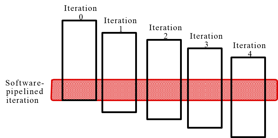
Software pipelining is a loop transformation technique that overlaps the execution of instructions from different iterations of a loop.
Rather than replicating the loop body, software pipelining schedules stages of different iterations into a single loop iteration. It effectively builds a pipeline where instructions from various iterations are executed in parallel, improving throughput without increasing code size significantly.
For instance, take the following loop:
for(i = 0; i < 5; i++) { A[i] = B[i]; // stage x A[i] = A[i] + 1; // stage y C[i] = A[i]; // stage z}
This loop has intra-iteration dependencies but no loop-carried dependencies. It can be transformed into a pipelined version by reorganizing stages:
This reorganization allows instructions from different iterations to be issued simultaneously, mimicking a hardware pipeline.
Software pipelining offers several advantages over loop unrolling. It typically results in smaller code size, since it avoids body duplication. Moreover, it fills and drains the pipeline only once for the entire loop, whereas loop unrolling fills and drains the pipeline for each unrolled block. Additionally, software pipelining can be combined with loop unrolling for further performance benefits, especially on architectures with deep pipelines or multiple functional units.
Trace Scheduling and Superblock Scheduling
When the loop body consists of a single basic block, software pipelining is an effective technique for maximizing parallelism. However, when the loop contains internal control flow, more advanced strategies are required to achieve efficient scheduling.
Definition
Global scheduling refers to the process of compressing a fragment of code with branches into a compact sequence of instructions, while preserving both data and control dependencies. This requires moving instructions across branch boundaries, something local techniques alone cannot handle.
A fundamental technique in this context is trace scheduling, which aims to identify and optimize likely execution paths across conditional branches. This technique consists of two main phases:
Steps
trace selection, where the most frequently executed sequence of basic blocks (the trace) is identified—using static analysis or profiling
trace compaction, where the trace is packed into a tight sequence of Very Long Instruction Word (VLIW) instructions to exploit available parallelism.
Since this scheduling is speculative, the compiler must also generate compensation code to handle cases where the actual execution flow deviates from the predicted one. This introduces overhead in terms of both register usage and execution time, as incorrectly speculated instructions must be undone or corrected.
An extension of trace scheduling is superblock scheduling, which further simplifies global optimization.
Definition
A superblock is defined as a group of basic blocks with a single entry point and multiple exit points, but no side entrances.
Superblocks are built using profiling information, often through tail duplication, which eliminates incoming control paths from outside the main trace. This transformation allows the compiler to avoid generating compensation code for entry points and focus only on exits. As a result, code within the superblock can be optimized more easily and effectively, since there is no external interference during the execution of the scheduled instructions.