8.1 - Recurrent Neural Network

Sequence Modeling

In the study of machine learning, sequence modeling focuses on handling dynamic datasets, which evolve over time, unlike the static datasets often used in conventional tasks. Dynamic data arises in numerous domains, including time series analysis, natural language processing, and signal processing. Modeling these sequences requires strategies to account for temporal dependencies and evolving patterns. Two broad categories of approaches address this challenge: memoryless models and models with memory.

Memoryless Models for Sequence Modeling

Memoryless models operate under the assumption that only a fixed number of previous observations (a fixed lag) are necessary to predict the next value in a sequence. This approach eschews the need for a comprehensive memory of past data and instead focuses on recent temporal windows. Key examples of memoryless models include autoregressive models and feedforward neural networks.

1. Autoregressive Models
   These models predict the next element in a sequence by linearly combining a fixed number of past inputs, known as delay taps. This structure restricts predictions to be a function of a limited history, effectively defining a fixed lag. Mathematically, these models are simple yet effective for capturing linear dependencies in data.

2. Feedforward Neural Networks
   Expanding on the principles of autoregressive models, feedforward neural networks incorporate non-linear transformations via hidden layers. By doing so, they can learn complex patterns and relationships in sequences. When augmented with delay taps, these networks use recent inputs and outputs to make predictions. The introduction of non-linearity makes feedforward networks a more general and powerful tool compared to their linear counterparts.

Dynamical Systems: Models with Memory

Unlike memoryless models, dynamical systems explicitly maintain an internal representation of the system’s state, capturing the entire historical context necessary for prediction. These models rely on a hidden state, which evolves over time according to specified dynamics. This hidden state, which cannot be observed directly, interacts with inputs to produce the sequence outputs. Dynamical systems are particularly suited for scenarios where long-term dependencies and noise are integral to the data.

1. Linear Dynamical Systems (LDS)
   In these systems, the hidden state is continuous and is assumed to follow Gaussian distributions. State transitions and the relationship between the state and observations are linear transformations. The Kalman filter, a cornerstone algorithm in control theory, is used to estimate the hidden state by combining noisy observations with the model’s internal dynamics. This makes LDS particularly effective in applications such as signal processing and robotics.

2. Hidden Markov Models (HMMs)
   Hidden Markov Models assume that the hidden state is discrete, transitioning stochastically between states according to a predefined transition matrix. Outputs are generated as probabilistic functions of the hidden states, often modeled through emission probabilities. Inference in HMMs is performed using algorithms like the Viterbi algorithm for determining the most likely sequence of states. HMMs are widely used in speech recognition and bioinformatics due to their ability to model sequential data with clear state transitions.

Recurrent Neural Networks (RNNs)

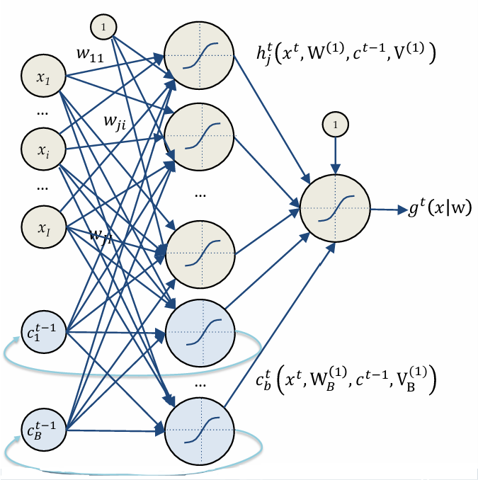
Recurrent Neural Networks (RNNs) are a class of neural networks specifically designed for sequence modeling, where temporal dynamics and dependencies between elements in a sequence are critical. Unlike feedforward networks, RNNs introduce memory through recurrent connections, allowing them to retain information about previous inputs while processing new ones. This structure enables RNNs to handle tasks where the output depends not only on the current input but also on the context provided by past inputs.

Memory and Computation in RNNs

The memory in RNNs is distributed across their hidden state, which evolves over time through non-linear updates. This capability to store and transform information efficiently allows RNNs to model complex patterns in sequential data. A remarkable property of RNNs, as described by Hava T. Siegelmann in 1995, is their theoretical ability to compute any function that can be executed by a computer, given enough time and computational resources. The hidden state dynamics in RNNs are governed by mathematical formulations like the following:

These equations represent how the current hidden state is updated based on inputs and the previous hidden state.

Backpropagation Through Time (BPTT)

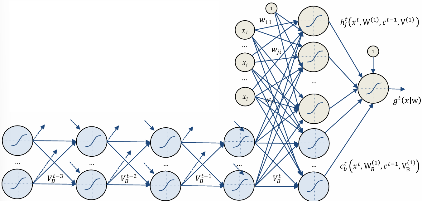
Training RNNs involves a specialized version of the backpropagation algorithm called Backpropagation Through Time (BPTT). This method unfolds the network across several time steps, treating it as a deep feedforward network. Gradients are computed for the unfolded network, ensuring that the parameters remain consistent across time steps. The updates to weights and can be expressed as:

However, BPTT faces challenges in training RNNs on long sequences due to the vanishing gradient problem, a phenomenon where gradients shrink exponentially as they propagate backward through time.

This issue arises because the gradients of the hidden states are repeatedly multiplied by small values, as shown:

If , the gradients tend to vanish, making it nearly impossible to learn long-range dependencies. This problem is particularly acute with activation functions like sigmoid or tanh, which have derivatives that rapidly shrink towards zero. To mitigate the vanishing gradient issue, researchers have explored several strategies:

1. ReLU Activation Function
   ReLU (Rectified Linear Unit) activation functions are used to force gradients to remain stable. ReLU is defined as:

   This ensures gradients are either 1 or 0, avoiding exponential decay.

2. Specialized Architectures
   Modern RNN variants, such as Long Short-Term Memory (LSTM) networks and Gated Recurrent Units (GRUs), incorporate small memory modules specifically designed to retain information over long sequences. These architectures use gating mechanisms to control the flow of information, thereby overcoming the limitations of simple RNNs.

Long Short-Term Memory (LSTM)

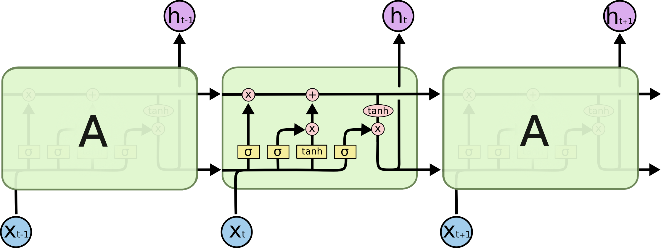
In 1997, Hochreiter and Schmidhuber proposed the Long Short-Term Memory (LSTM) architecture to address the vanishing gradient problem that plagued traditional Recurrent Neural Networks. LSTMs introduce a novel memory cell structure that enables the network to retain information over long time periods. The design relies on three key gates—input, forget, and output—which regulate the flow of information into, out of, and within the memory cell. These gates leverage multiplicative interactions and a combination of logistic (sigmoid) and linear units to ensure efficient storage and retrieval of information.

The three primary mechanisms in an LSTM are as follows:

• Write (Input) Gate: Controls when new information is written to the memory cell.
• Keep (Forget) Gate: Determines whether to retain or discard information stored in the memory cell.
• Read (Output) Gate: Facilitates reading stored information from the cell.

The fixed weights in the cell’s self-loop allow gradients to propagate through time effectively, avoiding the vanishing gradient problem and enabling stable learning of long-range dependencies.

Components of an LSTM

1. Input Gate
   The input gate decides how much of the new input information should be written to the memory cell. The activation of the input gate and the candidate cell state are computed as:

2. Forget Gate
   The forget gate determines which information from the previous cell state should be retained. It is computed as:

3. Memory Update
   The new cell state combines retained information from the previous state and the updated information from the input gate:

4. Output Gate
   The output gate controls what portion of the cell’s current state contributes to the hidden state . These are calculated as:

Gated Recurrent Unit (GRU)

The Gated Recurrent Unit (GRU) is a streamlined alternative to LSTMs. Introduced to simplify the architecture, GRUs combine the input and forget gates into a single update gate. Additionally, GRUs unify the memory cell state and the hidden state into a single entity. These simplifications reduce computational complexity while retaining the capability to model long-term dependencies effectively.

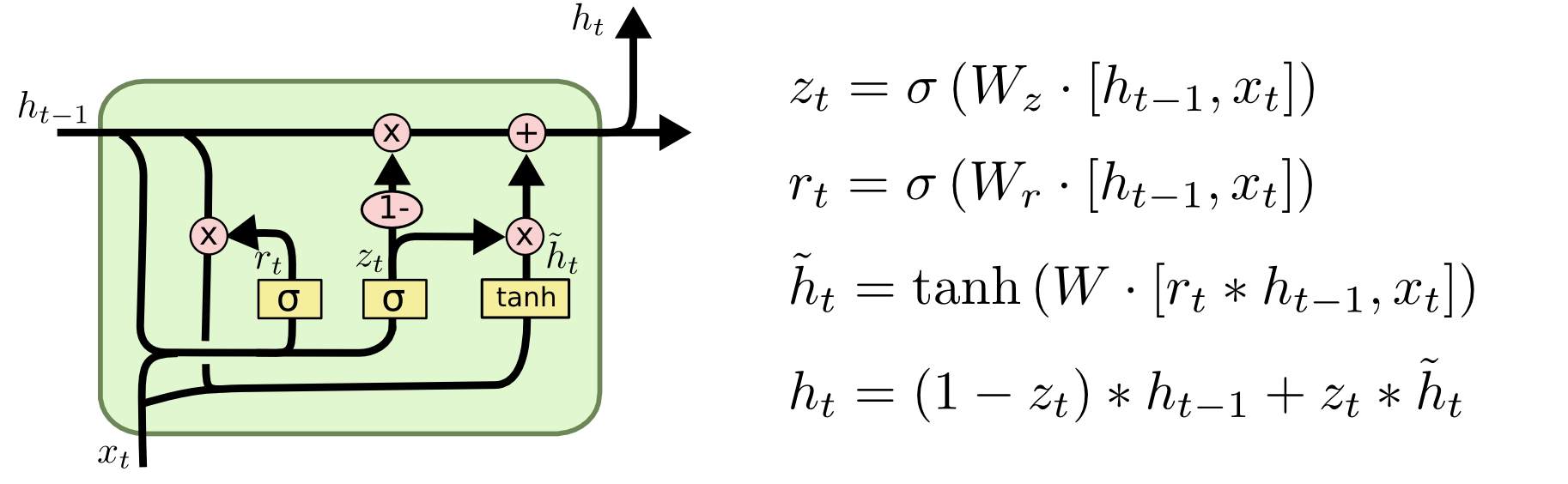
The GRU equations are:

1. Update Gate
   The update gate determines the balance between retaining past information and incorporating new inputs:

2. Reset Gate
   The reset gate decides how much of the previous state should influence the candidate activation:

3. Candidate Hidden State
   The candidate hidden state is computed using the reset gate :

4. Hidden State Update
   The final hidden state is a combination of the previous hidden state and the candidate hidden state, weighted by the update gate:

RNNs vs. LSTMs vs. GRUs

• RNNs struggle with long-term dependencies due to vanishing gradients, making them effective only for short sequences.
• LSTMs introduce a robust memory cell that overcomes the limitations of RNNs, enabling the modeling of complex, long-term dependencies.
• GRUs simplify LSTMs, offering a balance between computational efficiency and performance, with fewer parameters to train.

In practice, the choice between these architectures often depends on the dataset and computational constraints. While LSTMs are more expressive, GRUs are faster to train and perform comparably in many applications.

LSTM Networks and Computation Graphs

LSTM networks leverage computation graphs with continuous transformations to handle complex sequential data. This structure enables efficient modeling of dependencies over extended time periods, a critical improvement over traditional RNNs.

For tasks involving full input sequences, Bidirectional RNNs enhance the representation by incorporating context from both past and future inputs:

• One RNN processes the sequence in a left-to-right direction.
• Another RNN processes it in a right-to-left direction.
• Their hidden states are concatenated to form a more informative feature representation.

The initialization of the recurrent network’s state significantly impacts its performance:

1. Fixed Initialization: A simple approach where the initial state is set to a constant value, such as zero.
2. Learned Parameters: A more effective strategy involves treating the initial state as trainable parameters:
   • These states are initialized randomly and updated during training.
   • Gradients are propagated through time back to these parameters during training using gradient descent.
   • This approach allows the network to optimize its starting point for better performance.

Sequential Data Problems and Applications

Sequential data problems arise when both inputs and outputs are sequences of varying or fixed lengths. They are prevalent in diverse domains like natural language processing, vision, and audio processing.

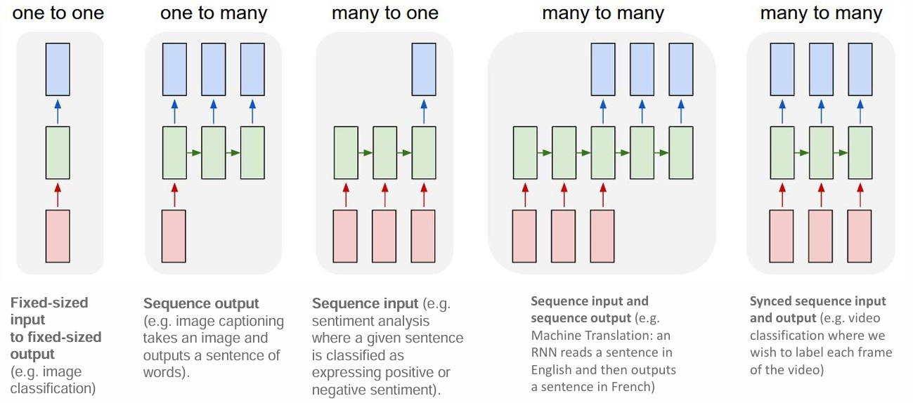
Model	Description	Example Task	Example Model
Model 1: One-to-One	A fixed-sized input is mapped to a fixed-sized output. This is the standard feedforward architecture used for tasks that require classification or regression.	Image classification (e.g., classifying handwritten digits with MNIST).	A convolutional neural network (CNN) with a softmax output layer.
Model 2: One-to-Many	A fixed-sized input is mapped to a sequence of outputs. This type of architecture is used for tasks where a single input generates a sequence of outputs.	Image captioning (e.g., generating a descriptive caption for an image).	A CNN extracts features from the image, followed by an RNN or Transformer to generate the caption.
Model 3: Many-to-One	A sequence of inputs is mapped to a single output. This architecture is used for tasks requiring summarization or classification of sequences.	Sentiment analysis (e.g., classifying a movie review as positive or negative).	An RNN or LSTM processes the sequence of words in the review and outputs the sentiment label.
Model 4: Many-to-Many (Sequence-to-Sequence)	A sequence of inputs is mapped to a sequence of outputs. This architecture is common in tasks where the output sequence differs in length or meaning from the input sequence.	Machine translation (e.g., translating an English sentence into French).	An encoder-decoder architecture using RNNs or Transformers.
Model 5: Many-to-Many (Synced Sequence)	A sequence of inputs is mapped to a sequence of outputs, where the input and output sequences are of the same length and aligned.	Video frame labeling (e.g., classifying the activity in each frame of a video).	An RNN processes the video frames, and an output is generated for each frame.

Sequence-to-Sequence Learning Examples

1. Image Captioning

   • Input: A single, fixed-size image.
   • Output: A variable-length sequence of words describing the image.
   • This task involves visual feature extraction (e.g., CNNs) followed by sequence generation using RNNs or LSTMs.

2. Sentiment Classification/Analysis

   • Input: A sequence of words or characters, such as a tweet or review, which can vary in length.
   • Output: A fixed-sized label, such as “positive” or “negative.”
   • This task often uses RNNs or transformers to encode the sequence into a fixed-size representation suitable for classification.

3. Language Translation

   • Input: A sequence of words in one language (e.g., English).
   • Output: A sequence of words in another language (e.g., French).
   • Both input and output sequences can have varying lengths, necessitating encoder-decoder architectures with attention mechanisms to align source and target tokens effectively.

---

References

• Understanding LSTM Networks — colah’s blog