8.2 - Seq2seq and Word Embedding

Language models are foundational in natural language processing, serving to estimate the probability of a sentence or sequence of words. Mathematically, the probability of a sequence is expressed as the product of the conditional probabilities of each word given the preceding words. This relationship is captured by:

This formulation highlights the sequential dependency of words in a sentence, where each word is predicted based on the words preceding it. Conditional language models extend this idea by incorporating an additional source of information, often another sequence or input, denoted as . The probability distribution in this context is given by:

In tasks like image captioning, the input sequence can be replaced with features extracted from an image , effectively adapting the conditional language model to operate with visual inputs instead of textual ones. This capability makes language models versatile tools across domains, from text generation to multimodal tasks.

Sequence-to-Sequence Modeling Basics

The goal of sequence-to-sequence modeling is to transform an input sequence into a target output sequence . The aim is to find the output sequence that maximizes the conditional probability . This can be formally expressed as:

In practical implementations, sequence-to-sequence models are trained on data to learn a probabilistic function , where represents the model parameters. During inference, the model predicts the output sequence by solving:

This approach is employed in a wide range of applications, including language translation, summarization, and speech recognition.

Machine Translation: Humans vs. Machines

Machine translation is a classical example of sequence-to-sequence modeling. In human translation, the probability of a translated sentence given an input sentence is based on the translator’s expertise and understanding of the language. This process can be expressed intuitively as:

For machine translation, however, this task is formalized as:

where, represents the learned parameters of the model. Machine translation involves three key components:

Modeling: Defining the functional form of , which may involve architectures such as recurrent neural networks (RNNs), transformers, or attention-based models.
Learning: Estimating the parameters by training the model on a dataset of aligned source and target sentences.
Search: Employing algorithms like beam search to efficiently find the output sequence that maximizes the conditional probability.

Each of these components poses its own challenges. For example, modeling requires balancing expressive power and computational efficiency, learning demands robust optimization techniques, and search strategies must navigate the exponential size of the output space.

The Encoder-Decoder Framework in Sequence-to-Sequence Models

The encoder-decoder framework forms the foundation of sequence-to-sequence models, which are widely used in tasks like machine translation, text summarization, and image captioning. True to the nature of most deep learning models, the encoder-decoder architecture maps an input sequence to an output sequence through a structured learning process.

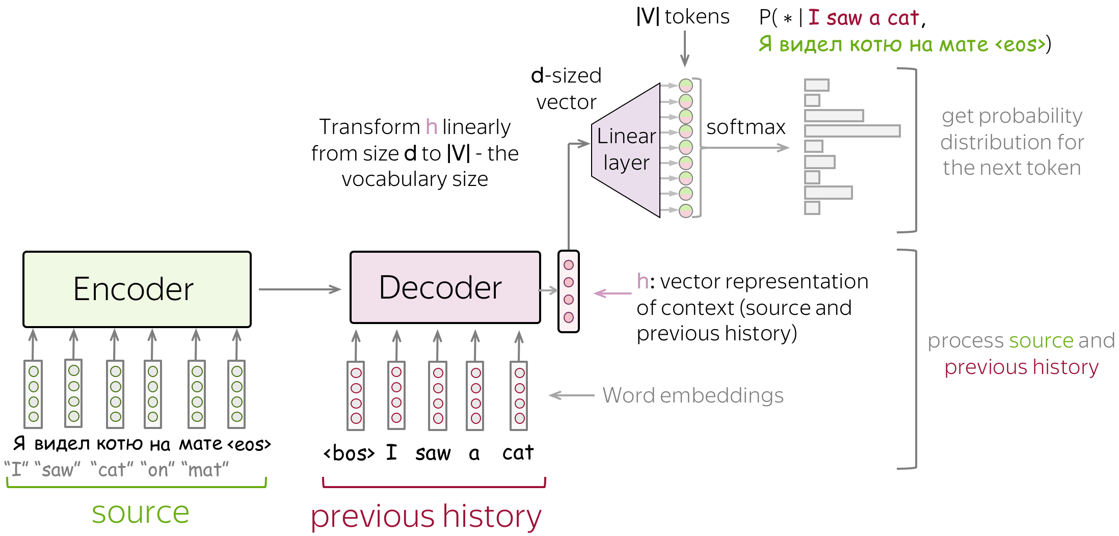
In this architecture, the encoder processes the input sequence into a fixed-length representation, often referred to as a “context vector.” This representation captures the salient information from the input sequence. The decoder then takes this context vector and generates the output sequence , one token at a time. While encoding and decoding can be performed using various neural architectures, recurrent neural networks (RNNs), particularly long short-term memory (LSTM) networks, have historically been a popular choice due to their ability to model sequential dependencies effectively.

Encoding and Decoding with Recurrent Neural Networks (LSTM)

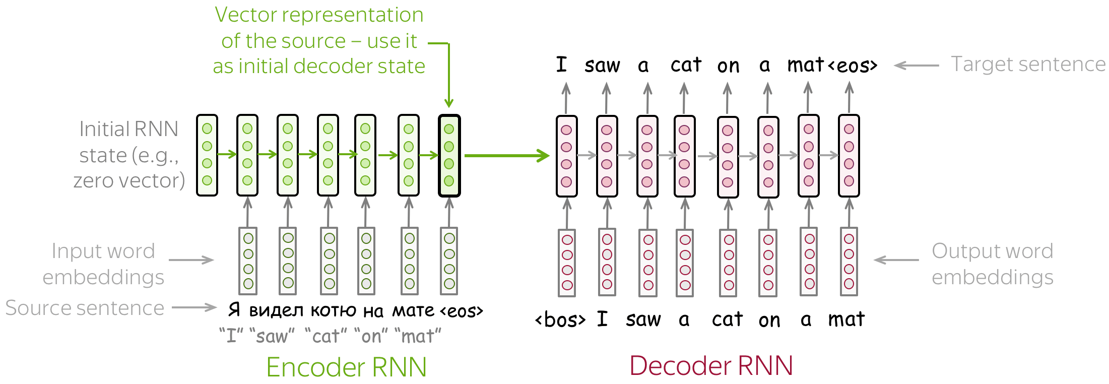
In the encoder-decoder setup, RNNs or LSTMs are employed to handle sequential data efficiently. The encoder, often implemented as a bidirectional LSTM, processes the input sequence and encodes it into a dense vector representation. This vector acts as a summary of the input sequence.

The decoder, also an LSTM, generates the output sequence conditioned on this vector and the tokens produced so far. At each decoding step , the decoder predicts the next token based on the previous outputs , the encoded input , and the model parameters . This step is governed by the conditional probability:

The sequential nature of this approach allows the decoder to dynamically adapt its predictions based on the context provided by both the encoder and its own past outputs.

Greedy Decoding vs. Beam Search

Once the model has been trained and the parameters have been learned, the task shifts to generating an output sequence for a given input sequence . This involves selecting the sequence that maximizes the conditional probability:

However, finding the optimal sequence requires an exhaustive search over all possible output sequences, which is computationally infeasible. To address this, two approximate decoding strategies are commonly used:

Greedy Decoding

In greedy decoding, the algorithm selects the most probable token at each step , without considering alternative sequences. This simplifies the search process:

While computationally efficient, greedy decoding is prone to suboptimal outputs because it cannot backtrack to correct early mistakes. Once a suboptimal token is chosen, it propagates through the rest of the sequence, potentially degrading the overall quality of the output.

Beam Search

Beam search addresses the limitations of greedy decoding by maintaining multiple hypotheses at each step. Instead of selecting a single token, the algorithm keeps track of the top most probable partial sequences (beams) and expands them in parallel. This approach allows the search to explore a larger portion of the solution space, increasing the likelihood of finding a better sequence. At the end of decoding, the most probable sequence among all beams is selected as the final output.

Beam search provides a balance between computational efficiency and output quality, making it a popular choice in real-world sequence-to-sequence applications. The trade-off lies in the choice of the beam width , where larger values improve the quality of results at the cost of increased computational complexity.

Training Sequence-to-Sequence Models

Training a sequence-to-sequence (Seq2Seq) model involves teaching the model to map input sequences to target sequences . At each time step , the model predicts the probability distribution , where:

This prediction relies on the previous outputs from the decoder and the input sequence encoded by the encoder. The target token is represented as a one-hot vector, and the cross-entropy loss is used to compute the error at each time step. The loss at a single time step is given by:

Here, represents the size of the vocabulary. Over the entire sequence, the total loss becomes:

This cumulative loss is minimized during training, enabling the model to learn parameters that best align predictions with the actual targets .

Seq2Seq: Training vs. Inference Time

Seq2Seq models follow the encoder-decoder architecture, where the training and inference processes differ significantly:

Training Time: During training, the decoder is conditioned on the actual target tokens rather than its previous outputs. This teacher forcing technique ensures that the decoder learns the correct mapping from the context vector and the ground truth sequence.
Inference Time: At inference, the decoder does not have access to the ground truth. Instead, it uses its own outputs as inputs for subsequent time steps. This iterative process is challenging because errors in earlier predictions can propagate and affect future steps.

Special Characters in Seq2Seq Models

Special tokens are essential in Seq2Seq models to handle practical challenges during training and inference. Commonly used special characters include:

<pad>: This token is used to pad shorter sequences in a batch so that all sequences have equal length. Padding ensures efficient computation but does not carry meaningful information.
<eos> (End of Sentence): Used in both source and target sequences to mark the end of a sentence. This helps the decoder determine when to stop generating tokens during inference.
<unk> (Unknown): Replaces out-of-vocabulary (OOV) tokens, improving efficiency by ignoring rare words that would otherwise inflate the vocabulary size.
<sos> or <go> (Start of Sequence): Marks the start of the target sequence and serves as the input to the first decoding step.

Dataset Batch Preparation

Preparing batches for training involves several preprocessing steps to standardize input and output sequences:

Sample a batch of pairs of .
Append <eos> to the end of each source sequence to mark sentence termination.
Prepend <sos> to the target sequence to form the input to the decoder and append <eos> to form the target output sequence.
Pad sequences in the batch to match the length of the longest sequence using <pad>.
Encode tokens into numerical representations using a vocabulary or embedding lookup.
Replace OOV tokens with <unk>.
Compute the length of each sequence for efficient masking during training.

For example, a vocabulary might be represented as:

Vocabulary = {
    "<sos>": 0,
    "<eos>": 99,
    "<unk>": 1,
    "<pad>": 3,
    "the"  : 42,
    "is"   : 16,
    ...
}

Numbers are assigned to tokens based on a predefined dictionary or frequency analysis, ensuring that each token has a unique ID for efficient processing.

Word Embeddings in NLP

Natural language processing often treats words as discrete atomic symbols. For example, “cat” might be encoded as ID 537, while “dog” is ID 143. However, this representation does not capture the semantic relationships between words. To address this, word embeddings are used.

Word embeddings map discrete tokens to dense, continuous vector spaces, enabling the model to learn semantic relationships like similarity and analogy. This transformation significantly enhances the ability of Seq2Seq models to understand and generate coherent sequences.

The encoding of text is fundamental to the performance of real-world NLP applications, such as chatbots, document classifiers, and information retrieval systems. Text encoding directly influences how well a system can understand, process, and respond to human language. Text representations can broadly be categorized into two types: local representations and continuous representations.

Local Representations

Local representations treat words as discrete entities, relying on statistical relationships in the immediate context of text. Common approaches include:

N-Grams Language Models: These models calculate the probability of a sequence using the chain rule:

In practice, n-gram models simplify this by assuming that the probability of a word depends only on the preceding words:

However, this approach requires smoothing techniques, such as Katz smoothing, to address zero probabilities caused by unseen word combinations in the training data.
Bag-of-Words (BoW): Represents text as a collection of unique words, disregarding word order but retaining frequency information. This approach is simple but lacks contextual nuance.
1-of-N Encoding: Each word is represented as a one-hot vector in a vocabulary-sized vector space, where only one entry (corresponding to the word) is set to 1, and all others are 0. This representation is efficient for small vocabularies but scales poorly for large datasets.

Continuous Representations

Continuous representations aim to overcome the limitations of local models by capturing deeper semantic relationships:

Latent Semantic Analysis (LSA): A technique that uses matrix factorization to uncover the latent structure in a corpus, identifying relationships between terms and documents.
Latent Dirichlet Allocation (LDA): A generative probabilistic model that represents documents as mixtures of topics, with each topic characterized by a distribution over words.
Distributed Representations (Word Embeddings): These encode words into dense, low-dimensional vectors that capture semantic similarity. Unlike one-hot vectors, embeddings reflect relationships, such as synonyms and analogies.

Challenges of N-Gram Language Models

Despite their simplicity, n-gram models suffer from significant drawbacks.

First, there is the curse of dimensionality. A -gram model on a corpus with unique words operates in a 10-dimensional hypercube with slots. Assigning probabilities to such a vast space requires enormous amounts of data, which is impractical. Larger corpora bring more unique words, exacerbating the sparsity problem.

Second, n-gram models have limited context. In practice, n-grams often use a context of size 2 or 3 (e.g., trigram models), as longer contexts are computationally expensive and data-hungry. Short contexts fail to capture long-range dependencies, resulting in loss of semantic information.

Third, n-gram models ignore word similarity. One-hot vectors and classic n-gram models treat each word as independent and unrelated. Consider the sentences: “Obama speaks to the media in Illinois.” and “The President addresses the press in Chicago.” Classic models represent these sentences as: , , , , , . These representations fail to capture similarities (e.g., “Obama” and “President”) or semantic relationships (e.g., “Illinois” and “Chicago”). Words in these models are orthogonal, making it impossible to generalize based on semantic similarity.

Moving Beyond N-Grams

To address the limitations of n-gram models, NLP has transitioned to using distributed representations, such as word embeddings (e.g., Word2Vec, GloVe). These representations embed words into a continuous vector space where similar words have similar vector representations. For example:

“Obama” and “President” would have embeddings close to each other.
“Illinois” and “Chicago” would be related in their spatial positions.

This shift has enabled models to generalize better, understand context more effectively, and overcome the sparsity and dimensionality issues inherent in classic models.

Word Embeddings: Mapping Words to Numerical Representations

Word embeddings are computational techniques that map words or phrases from their original high-dimensional space (the set of all words in a language) into a lower-dimensional numerical vector space. This process embeds the word in a compact and meaningful representation, where the spatial relationships between the vectors encode semantic relationships between words. In this vector space, words with similar meanings or contextual usage are represented as points that are closer to each other, often forming distinct clusters.

Neural Autoencoders for Embeddings

One approach to generating embeddings is through neural autoencorder, a type of neural network trained to reproduce its input. The network includes an encoder that compresses the input into a low-dimensional hidden representation and a decoder that reconstructs the input from this representation. This process forces the network to capture the most salient features of the input in a condensed form.

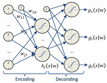
Formally, the autoencoder maps an input to a compressed representation , where . The decoder then maps back to the reconstructed output . The training objective minimizes the reconstruction error while enforcing sparsity in the hidden layer:

The first term measures how accurately the input is reconstructed, while the second term imposes sparsity, ensuring that only a small number of neurons are active, which aids in learning a compressed, meaningful representation.

Distributed Representations of Words

Distributed word representations, or word embeddings, map each word in a large vocabulary (where ) to a continuous -dimensional space, with typically. This representation combats the curse of dimensionality by employing techniques such as:

Compression: Reducing the dimensionality of the representation.
Smoothing: Transforming discrete representations into continuous ones.
Densification: Transitioning from sparse, one-hot encodings to dense vector representations.

By mapping words into this compact space, semantically similar words are placed closer together, enabling models to generalize better across linguistic contexts.

Neural Network Language Model (NNLM)

In 2003, Bengio et al. proposed the Neural Network Language Model (NNLM), which integrates word embeddings into language modeling tasks. The model includes a projection layer that contains the word vectors . Given a context window of two words, the model predicts the next word using these embeddings.

The computational complexity of training this model using stochastic gradient descent is , where is the context window size, is the embedding dimension, is the number of hidden units, and is the vocabulary size.

Bengio et al. primarily focused on improving the accuracy of language models, leaving the optimization of word vectors as a secondary concern. However, subsequent research, particularly by Mikolov et al. (2013), shifted the focus to optimizing word vectors, leading to significant advancements in embedding quality.

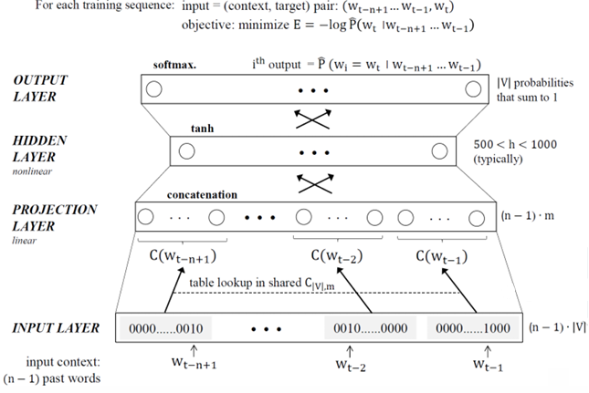
Softmax is used to output a multinomial distribution

is the concatenation of the context weight vectors
is the projection-to-hidden weights matrix
and are biases (respectively and elements)
is the matrix with hidden-to-output weights

Despite its contributions, the NNLM faced several challenges. Training was computationally intensive due to the need to process large vocabularies and model complexities. For instance, training on datasets like the Brown Corpus ( million words, vocabulary size ) and AP News ( million words, vocabulary size , reduced to ) required weeks of computation on 40 CPU cores. Moreover, NNLMs struggled to handle rare words effectively due to limited data availability for such tokens.

The introduction of simpler, more scalable methods like Word2Vec (Mikolov et al., 2013) addressed many of these limitations, revolutionizing the field of word embeddings and enabling widespread application in natural language processing tasks.

Google’s Word2Vec: Revolutionizing Word Embeddings

In 2013, Mikolov et al. introduced word2vec, a groundbreaking approach to word embeddings. Unlike earlier neural network-based language models, Word2Vec uses a simpler, shallower model to process much larger datasets efficiently. This simplification eliminates the need for a hidden layer, resulting in a 1000x speed improvement over previous methods. Additionally, Word2Vec shares a projection layer, unlike traditional models that only share the weight matrix. It takes advantage of both historical and future context for predicting words, echoing John R. Firth’s famous linguistic principle: “You shall know a word by the company it keeps.”

The Continuous Bag-of-Words (CBOW) Model

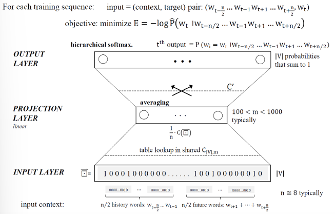
One of Word2Vec’s two primary architectures is the Continuous Bag-of-Words (CBOW) model. CBOW predicts a target word based on the context words surrounding it. During training, only the vectors for context words are updated for each training pair . If the predicted probability of a target word is overestimated, the algorithm subtracts a portion of the context word vectors in the matrix . Conversely, if the probability is underestimated, the algorithm adds a portion of the target word vector to the context word vectors, refining the embeddings iteratively.

Word2Vec dramatically improved upon the complexity of earlier Neural Network Language Models (NNLMs). The complexity of CBOW is approximately , where:

: Context window size
: Embedding dimension
: Vocabulary size

For example, training Word2Vec on a 6-billion-word Google News dataset (with a vocabulary size of approximately ) was completed in just 2 days using 140 CPU cores for CBOW (embedding dimension ). By comparison, NNLMs such as those introduced by Bengio et al. (2003) required 14 days on 180 cores for a much smaller . Moreover, Word2Vec achieved a training speed of words per second and surpassed NNLMs in performance, with Skip-Gram achieving % overall accuracy compared to NNLM’s %.

The Skip-Gram Model and Semantic Vector Spaces

Word2Vec’s other architecture, the Skip-Gram model, predicts context words given a target word. This approach is particularly effective for capturing semantic and syntactic relationships, even across longer contexts. The embeddings produced by Word2Vec support intuitive vector operations, demonstrating regularities in the embedding space. For instance:

These operations show how word embeddings encode meaningful relationships, making them invaluable for tasks requiring semantic understanding.

Applications of Word2Vec in Information Retrieval

Word2Vec has profound implications for information retrieval. For example, a query like “restaurants in Mountain View that are not very good” can be broken down into phrases such as “restaurants in (Mountain View) that are (not very good)”. These phrases can then be represented as continuous vectors, enabling models to capture semantic similarities between documents.

Unlike traditional bag-of-words (BoW) approaches that rely on exact word matches, Word2Vec embeddings encode semantic meaning, allowing for a richer understanding of text. By comparing cosine distances between document vectors, retrieval systems can determine document relevance without requiring explicit classifiers.

References

NLP Course | For You

Polimi CS - Notes

Explorer