In database management systems (DBMS), data needs to be stored in files on secondary memory devices (like hard drives or SSDs) for two primary reasons:
- Size: Databases often exceed the capacity of a system’s main memory (RAM), making it necessary to store data on larger, but slower, secondary memory.
- Persistence: Secondary memory ensures data is retained even after the system is powered off, offering durability and reliability that is critical for long-term data storage.
Since data resides in secondary memory, it cannot be used directly. The DBMS must first transfer this data into main memory before any operations (such as queries) can be performed on it. This introduces a concept central to the database cost model—I/O operations, which dominate the cost of data access.
Definitions
- Page: A unit of storage in main memory.
- Block: A unit of storage in secondary memory.
The DBMS organizes data in secondary memory into blocks, and when data is needed, an entire block is transferred between secondary and main memory as a page.
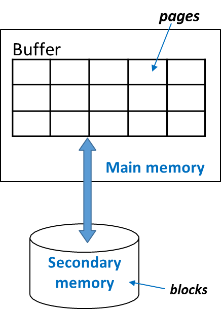
In most systems, the size of a page equals the size of a block, typically a few kilobytes (KB). However, some systems may allow a page to span multiple blocks.
Mechanical Hard Drives (HDDs) and Solid-State Drives (SSDs)
Definition
Mechanical hard drives consist of multiple disks (platters) stacked together, rotating at a constant angular speed. A head stack, mounted on an arm, moves radially to access tracks at different distances from the spindle (rotation axis). To read or write data, the drive waits for the desired sector to pass under one of the heads. Multiple blocks can be accessed simultaneously, corresponding to the number of heads/disks.
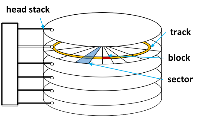
Accessing data on a mechanical hard drive involves three main components:
- Seek Time (8-12ms): The time required for the read/write head to move to the correct track.
- Latency Time (2-8ms): The delay caused by the rotation of the disk until the correct sector is aligned with the read/write head.
- Transfer Time (~1ms): The time taken to transfer data from the disk to main memory once the correct sector is aligned.
Accessing secondary memory is significantly slower than accessing main memory, with costs being approximately four orders of magnitude higher.
In “I/O bound” applications, the performance cost is primarily determined by the number of accesses to secondary memory. Therefore, the cost of executing a query is directly proportional to the number of blocks that need to be transferred.
Definition
Solid-state drives, in contrast, do not have any moving parts, resulting in much faster read and write speeds compared to HDDs. The lack of mechanical components eliminates the need for seek and latency times.
As a result, SSDs can access data almost instantly, typically reducing data retrieval time to microseconds. However, SSDs are more expensive per unit of storage.
In databases, the performance of query execution is largely determined by the number of I/O operations required to access the necessary data blocks. Since I/O operations are slow, the DBMS typically employs strategies to minimize them:
- Buffering: Storing recently accessed pages in main memory so that future accesses can be served without performing additional I/O.
- Indexing: Using index structures that reduce the number of blocks that need to be read to find the desired records.
- Caching: Keeping frequently accessed data in memory to speed up queries.
DBMS and File System
Definition
The file system (FS) is a component of the OS that manages access to secondary memory.
While the file system provides an abstraction layer for storing and retrieving data, Database Management Systems typically make only limited and specific use of its functionalities. This selective utilization primarily encompasses basic operations such as creating and deleting files, along with reading and writing data blocks.
A significant distinction arises from the fact that a DBMS often assumes direct control over its internal file organization, extending beyond the high-level abstractions offered by the OS file system. This direct management encompasses the intricate details of record distribution within data blocks and the precise internal structure of each block. For instance, a DBMS might implement its own buffering and caching mechanisms to optimize I/O operations, bypassing certain OS file system caches.
Furthermore, advanced DBMS implementations may even manage the physical allocation of data blocks directly onto the disk. This fine-grained control allows the DBMS to optimize for various performance characteristics, such as achieving faster sequential reads by ensuring contiguous block allocation, gaining precise control over the execution time of write operations for performance-critical transactions, and enhancing overall data reliability through custom data placement strategies.
Physical Access Structures
In DBMSs, physical access structures are essential for managing how data is stored, retrieved, and updated. Each DBMS comes with a limited set of access methods, which are essentially software modules that define the primitives (basic operations) for interacting with different types of physical data structures. These methods handle both data organization and manipulation.
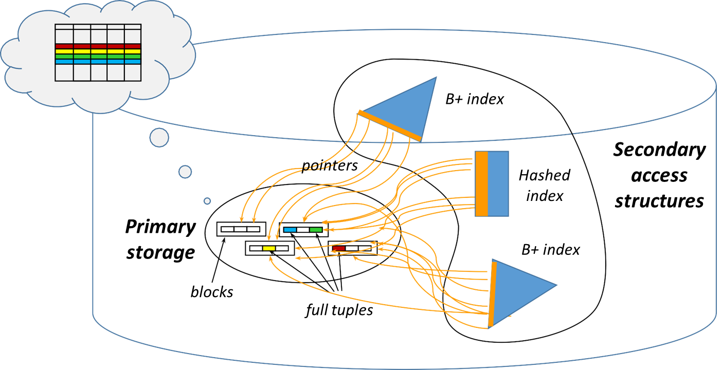
Every table in a database is stored within one primary physical structure and can be linked to one or more (optional) secondary access structures. The primary structure contains the actual data (tuples) of a table, whereas secondary structures—typically indexes—exist to facilitate faster access to data by creating shortcuts based on specific fields, known as search keys.
Primary and Secondary Structures
Definition
The primary structure is used mainly for storing the content of the table in a comprehensive and orderly way. On the other hand, secondary structures (indexes) are specifically designed to improve the efficiency of data retrieval by providing quick access to the primary structure. These secondary structures store only certain fields (such as search keys) along with pointers that direct the system to the corresponding blocks in the primary structure.
The primary purpose of the primary structure is to hold the complete set of tuples, whereas the main objective of secondary structures is to facilitate efficient searching based on specific criteria (like searching for all records where a field matches a given value).
There are three principal types of physical access structures:
- Sequential Structures: Data is stored and accessed in a linear order.
- Hash-Based Structures: Use hash functions to map data to a location.
- Tree-based structures: Use hierarchical structures (like B-trees) to index and access data.
Not all types of physical structures are suited for both primary and secondary storage.
| Type of Structure | Primary | Secondary | Comparison |
|---|---|---|---|
| Sequential structures | Typical | Rarely used | Simple, efficient for inserts and full scans; slow for searches unless ordered; best for bulk loads. |
| Hash-based structures | In some DBMSs (e.g., Oracle hash clusters) | Frequent | Fast point queries ( |
| Tree-based structures | Rare (obsolete) | Typical | Good for both point and range queries; supports ordered access; more complex and slower for inserts. |
Blocks and Tuples
In a database, blocks are the physical units of storage, while tuples (also known as records) are the logical units.
- Blocks represent fixed-size units (usually in kilobytes) determined by the file system and disk format.
- Tuples, however, vary in size based on database design and can have variable length depending on the data they hold, such as optional fields or variable-length attributes like
varchar.
Each block is organized into the following sections:
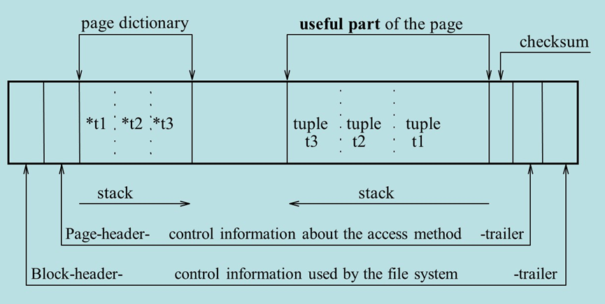
- Block header and trailer: Contain control information for the file system.
- Page header and trailer: Store metadata for the access method used.
- Page dictionary: Holds pointers (an offset table) to each piece of useful data within the block.
- Useful part: Contains the actual data (the tuples).
- Checksum: Ensures data integrity by detecting corrupted data.
The way tuples are organized within a block impacts the system’s ability to quickly retrieve or modify data.
The block factor (
Formula
To calculate the block factor, the following formula is used:
where:
= Average size of a tuple (assuming a fixed-length record). = Size of a block (in bytes). This formula determines how many tuples can fit into a block. If the block is not fully utilized, the remaining space may be wasted (in the case of unspanned records) or may be used by spanning the tuple across multiple blocks.
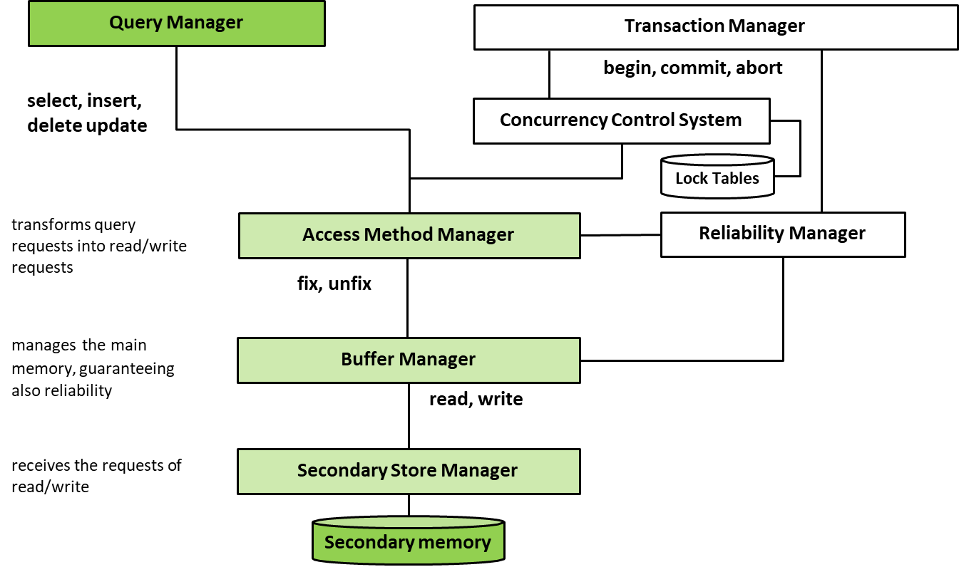
Buffer Management and I/O Operations
Definition
The buffer manager is responsible for handling I/O operations in memory, primarily by managing the pages, which are the in-memory equivalents of blocks.
The buffer manager decides when to bring pages from secondary storage (disk) to main memory (RAM) and when to write modified pages back to disk.
Key buffer manager primitives include:
- Insertion and Update: Adding or updating a tuple may involve reorganizing a page, especially for variable-length fields like
varchar. In some cases, it may require allocating new pages. - Deletion: Deleting a tuple typically involves marking it as invalid, followed by page reorganization at a later time.
- Field Access: Accessing a specific field in a tuple is done using an offset from the start of the tuple, based on the field’s position and length (stored in the page dictionary).
These operations must be optimized to minimize the number of costly I/O operations, which dominate the performance of query execution in most database systems.
Sequential Structures
Definition
Sequential structures refer to the arrangement of tuples (records) in secondary memory in a sequence that supports block-by-block access. These structures can be either contiguous or sparse in memory, with each block potentially spread across different areas of the disk.
There are two primary types of sequential structures:
- Entry-sequenced organization (also called heap)
- Sequentially-ordered organization
Comparison
Operation Entry-sequenced Sequentially-ordered INSERTEfficient (just append) Not efficient (requires reordering) UPDATEEfficient (if size increases, delete + insert) Not efficient if data size increases DELETEMarks the tuple as “invalid” Marks the tuple as “invalid” Tuple Size Fixed or variable Fixed or variable SELECT * FROM T WHERE key ...Inefficient (requires full scan) More efficient (leverages sorted order) Entry-sequenced organization is the most common solution, but PAIRED with secondary access structures
Entry-Sequenced Sequential Structure (Heap)
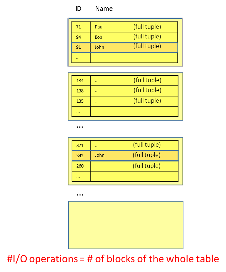
In an entry-sequenced structure, tuples are stored in the order they are inserted, without regard to the values of any particular key.
| Advantages | Disadvantages |
|---|---|
| Efficient for insertions: Since the data is simply appended to the end of the structure, new tuples can be inserted without needing to shift existing records. | Inefficient for searches: Querying specific tuples (e.g., SELECT * FROM Student WHERE Name = 'John') may require scanning the entire table, resulting in a high number of I/O operations unless a secondary index is in place. |
| Optimal space utilization: All available space is used, with no unused blocks or gaps. | Updates: If an update increases the size of a tuple, it may no longer fit in the original block. This requires either a shift or moving the tuple to another block, which adds overhead. |
| Efficient for sequential access: If the table is stored contiguously on disk, sequential scans (like SELECT * FROM table) can be performed quickly, with minimal disk seeks and latency. |
Example
For a query
SELECT * FROM Student WHERE Student.Name = 'John', we may need to scan through every block until the desired tuple is found.
The number of I/O operations is equal to the total number of blocks in the table, as every block must be checked.
Sequentially-Ordered Sequential Structure
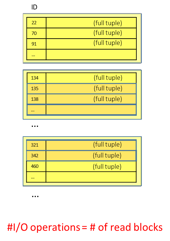
In a sequentially-ordered structure, tuples are ordered based on the value of one or more key fields. This makes it effective for range queries or any queries that involve sorting or grouping.
| Advantages | Disadvantages |
|---|---|
| Efficient for range queries: Queries that retrieve tuples based on a key interval (e.g., SELECT * FROM Student WHERE Student.ID BETWEEN '135' AND '380') benefit from the sorted order, making the query more efficient. | Insertions are less efficient: New tuples must be inserted in the correct order, which may require shifting existing tuples. In some cases, overflow files or differential files are used to temporarily store new tuples before periodically merging them into the main structure. |
| Optimized for sorting and grouping: Queries like ORDER BY and GROUP BY can leverage the already sorted data to improve performance. | Updates can be problematic: Updates that increase tuple size may necessitate moving the tuple to a new location, requiring reordering within the block or the use of overflow blocks. |
To avoid global reordering, several techniques are employed:
- Differential files: New data is added to a separate file and periodically merged with the main structure (e.g., like old yellow pages).
- Pre-allocated free space: Some space is left unused in each block to accommodate local reordering.
- Overflow files: When a block is full, new records are added to an overflow block, which is linked to the original block (common in many access structures).
Example
For the query
SELECT * FROM Student WHERE Student.ID BETWEEN '135' AND '380', only the blocks containing records within that range need to be accessed.
The number of I/O operations depends on the number of blocks that contain relevant data.
Hash-Based Structures
Hash-based structures provide a highly efficient mechanism for implementing associative access to data, making them a cornerstone of database indexing for queries that specify an exact key value. This indexing technique organizes data into a collection of buckets, where each bucket typically corresponds to one or more physical memory blocks. The core of the structure is a hash function, a deterministic mathematical function that computes a bucket address directly from a given key. This direct mapping allows the system to locate the data associated with a specific key in what is, on average, a constant amount of time, denoted as
The process of mapping a key to a bucket address involves two primary stages.
- First, if the key is not already a numeric type (e.g., if it is a character string), a folding step is applied to transform it into a positive integer. This initial transformation is designed to distribute the keys uniformly over a large numerical range.
- Following this, a hash function,
, is applied to the resulting integer. A common and simple hash function is the modulo operator, such as , where represents the total number of buckets in the hash table. This function maps the integer representation of the key to a bucket index in the range , determining the physical location where the corresponding tuple should be stored or retrieved.
The primary advantage of hash-based indexing lies in its exceptional performance for point queries, which are queries that use an equality predicate on the indexed key (e.g., WHERE key = value). Since the hash function directly calculates the bucket address, retrieval is typically achieved with a single I/O operation, assuming no collisions. However, this strength is also the source of its main limitation. The hash function intentionally scatters keys across the available buckets to ensure a uniform distribution, thereby destroying any natural ordering of the data. As a result, hash indexes are highly inefficient for processing range queries (e.g., WHERE key BETWEEN x AND y), as there is no correlation between key proximity and bucket location, forcing the system to scan all buckets. Furthermore, static hash structures perform optimally on relatively stable datasets.
In environments with high volumes of insertions and deletions, the number of tuples can change significantly, which disrupts the balance of the structure and can lead to performance degradation unless the entire hash table is periodically reorganized or a more advanced dynamic hashing technique is employed.
Example
Given the hash function
, a key would be mapped to bucket 1:
Collision Handling and Overflow Management
Definition
A collision occurs when the hash function maps two or more distinct keys to the same bucket address.
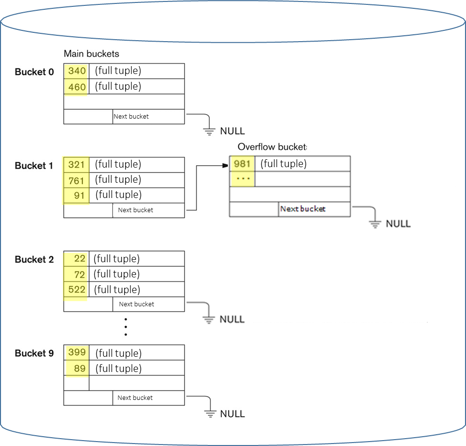
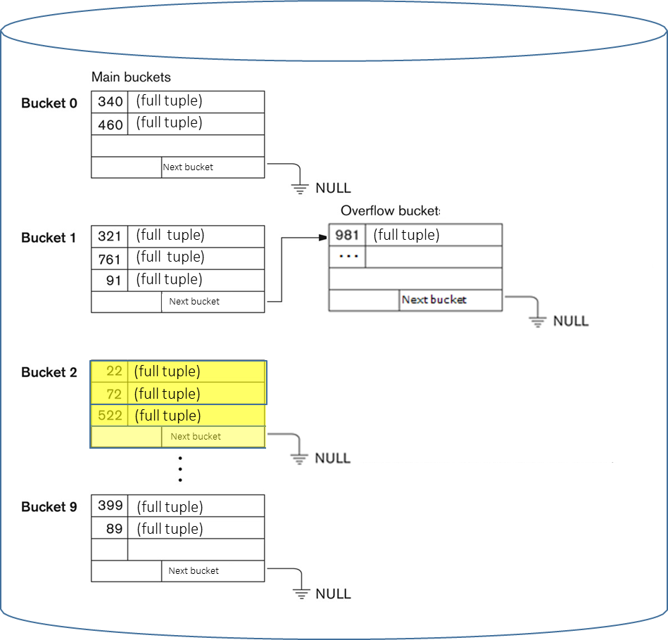
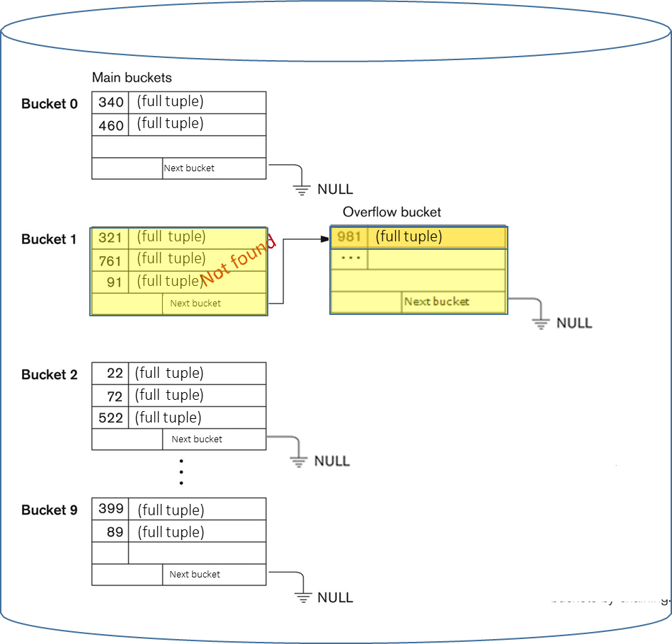
Because the number of possible keys typically far exceeds the number of available buckets, collisions are an inevitable aspect of hashing. The predominant method for handling collisions in database systems is open hashing, more commonly known as separate chaining. In this approach, each bucket acts as the head of a linked list. When a new tuple hashes to a bucket that is already full, an overflow bucket (an additional memory block) is allocated and linked to the primary bucket, forming an overflow chain. When searching for a key, the system first hashes to the primary bucket; if the desired tuple is not found there, it traverses the linked overflow chain sequentially. While effective, this process increases the number of I/O operations required for retrieval.
A less common alternative, closed hashing (or open addressing), attempts to resolve collisions by placing the colliding tuple in a different, nearby bucket according to a predefined probing sequence, but this method is rarely used in DBMSs due to its performance degradation at high load factors and complexities with deletion.
Example
Given the hash function
, consider the two following scenarios:
- If we have to perform the query
SELECT * FROM Student WHERE Student.ID = '522', the hash function computes. The system first checks bucket 2 and the number of I/O operations is 1 if the tuple is found there. - If we have to perform the query
SELECT * FROM Student WHERE Student.ID = '981', the hash function computes. The system first checks bucket 1. If the tuple is not found, it will traverse the overflow chain linked to bucket 1, requiring additional I/O operations (so the number of I/O operations is 1 from the main bucket plus the average length of the overflow chain).
The Load Factor and Performance Tuning
The efficiency of a hash-based structure is fundamentally governed by its load factor, a metric that quantifies how full the hash table is.
New formula
The load factor is calculated as:
where,
represents the total number of tuples in the table, is the block factor (the number of tuples that can be stored in a single block or bucket), and is the total number of buckets.
This ratio is critical for performance tuning.
- A low load factor (
) implies that buckets are sparsely populated, which wastes storage space but minimizes the probability of collisions and keeps overflow chains short or non-existent. - Conversely, a high load factor (
or ) indicates that buckets are nearly full or overflowing, which improves space utilization but significantly increases the average length of overflow chains and, consequently, the number of disk accesses required for search and insert operations.
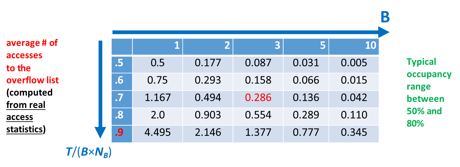
To balance these competing concerns, system administrators typically aim to maintain a bucket occupancy between 50% and 80%, which provides a practical compromise between efficient storage utilization and fast data access.