4.3 - Concurrency Control in Practice and Locking

Ensuring conflict-serializability while transactions are happening requires online concurrency control mechanisms. Unlike theoretical models that evaluate schedules a posteriori (after transactions have completed), real systems must make decisions in real-time. This poses several challenges:

Immediate Decision-Making: The scheduler must decide whether to execute, delay, or reject an operation as soon as it is requested.
Uncertainty of Transaction Commit: Not all transactions will commit. Many may abort, meaning that a concurrency control system cannot rely solely on committed schedules.
Efficiency: The mechanism must minimize overhead, avoiding performance degradation.

When analyzing concurrency, we distinguish between:

A Posteriori Schedules: The final order in which operations were executed by transactions, often referred to as a “history.” These are constructed after execution and can be analyzed for serializability or other properties.
Arrival Sequences: The sequence in which transaction operations are requested (before they are executed). The scheduler processes these in real-time to decide how to handle the concurrency.

In the realm of database concurrency control, the notation such as serves as a representation of a “schedule,” which fundamentally provides an a posteriori perspective on the execution flow of concurrent transactions within a DBMS. A schedule meticulously details the sequence of operations that have been performed by specific transactions on particular data items. The scope of a schedule can be narrowed through the application of the “commit-projection hypothesis.” This hypothesis posits that only operations executed by transactions that have successfully committed are relevant for consideration within the schedule. This restriction is crucial for analyzing the final, stable state of the database, as operations from aborted or uncommitted transactions are effectively undone and do not contribute to the persistent state.

While schedules offer a retrospective view, the field of “online” concurrency control necessitates the consideration of “arrival sequences.” These sequences represent the chronological order in which operation requests are issued by transactions. Unlike a schedule, an arrival sequence models the dynamic stream of incoming requests to the DBMS. Although there is a slight abuse of notation, where arrival sequences are sometimes represented in the same format as a posteriori schedules (e.g., ), the context in which these notations are used typically clarifies whether a retrospective schedule or a prospective arrival sequence is being described.

Concurrency Control Approaches

There are two major families of techniques for managing concurrency control in practice: Pessimistic and Optimistic.

Pessimistic Concurrency Control
- Locks: The most common method in pessimistic concurrency control is the use of locks. When a transaction wants to access a resource (such as a piece of data), it must acquire a lock on that resource. There are typically two types of locks:
  - Read locks (shared): Multiple transactions can hold read locks simultaneously, as long as no transaction writes to the resource.
  - Write locks (exclusive): Only one transaction can hold a write lock at a time, preventing others from reading or writing to the resource.
- Blocking: If a resource is already locked, the scheduler may block the transaction until the resource becomes available. This ensures that no conflicting operations occur but may introduce delays or deadlocks (when transactions block each other in a circular waiting pattern).
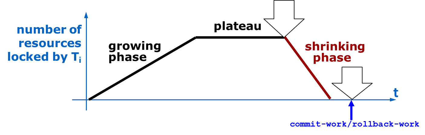
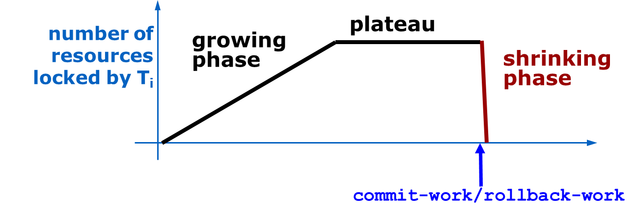
- Two-Phase Locking (2PL): A common locking protocol that guarantees serializability:
  - Growing Phase: A transaction acquires all the locks it needs.
  - Shrinking Phase: A transaction releases locks but cannot acquire any new ones after this point.

Aspect	Pessimistic Control
Benefits	- Strong guarantees: Avoids anomalies by ensuring that conflicting operations never occur simultaneously. - Suitable for high-contention environments: Prevents costly conflicts when many transactions access the same resources.
Drawbacks	- Overhead: Lock management can slow down transactions, especially in low-contention environments where conflicts are rare. - Deadlocks: Requires additional mechanisms to detect and resolve deadlocks.

Optimistic Concurrency Control
- Timestamp Ordering: In optimistic control, each transaction is assigned a timestamp when it starts. Operations are allowed to proceed without immediate checking for conflicts. At commit time, the scheduler checks if the transaction’s operations conflict with those of others. If a conflict is detected, the transaction is aborted and must restart. Some systems use versioning to allow transactions to read from older versions of the data while newer versions are being written. This allows more transactions to proceed in parallel without waiting for locks.
- Validation Phase: Before committing, the transaction undergoes a validation phase to ensure that its operations are serializable with respect to other concurrent transactions. If the validation fails, the transaction is aborted and must retry.

Aspect	Optimistic Control
Benefits	- Minimal Overhead: Transactions proceed without waiting for locks, making it effective in low-contention environments where conflicts are rare. - Concurrency: Multiple transactions can proceed in parallel without blocking each other.
Drawbacks	- Abort Rate: Frequent conflicts can lead to many transactions being aborted during the validation phase, resulting in wasted computation and reduced performance. - Validation Cost: The validation phase can be expensive as the system checks for conflicts at commit time.

Comparison of Approaches

Aspect Pessimistic Control Optimistic Control
Conflicts Avoided by locking resources upfront Handled at commit time (may abort)
Best suited for High-contention environments Low-contention environments
Overhead High (locking, deadlock detection) Low (only validation at commit)
Concurrency Lower (due to locks and blocking) Higher (more parallel execution)
Transaction Abort Rate Low (since conflicts are avoided) Higher (due to commit-time conflicts)

Aspect	Pessimistic Control	Optimistic Control
Conflicts	Avoided by locking resources upfront	Handled at commit time (may abort)
Best suited for	High-contention environments	Low-contention environments
Overhead	High (locking, deadlock detection)	Low (only validation at commit)
Concurrency	Lower (due to locks and blocking)	Higher (more parallel execution)
Transaction Abort Rate	Low (since conflicts are avoided)	Higher (due to commit-time conflicts)

Many commercial systems implement hybrid approaches that combine elements of both pessimistic and optimistic control to balance the strengths and weaknesses of each:

Adaptive Locking: Systems may start with optimistic control but switch to pessimistic control in high-contention scenarios.
Snapshot Isolation: A version of optimistic control where transactions work on “snapshots” of the database at the start of the transaction, reducing the need for locks but ensuring consistency.

Locking Mechanism in Concurrency Control

Definition

Locking is a core technique in pessimistic concurrency control that ensures transactions access shared resources (like data) without causing anomalies, such as dirty reads or lost updates. It controls the access to resources by enforcing locks (shared or exclusive) on them.

There are two primary types of locks:

Read Lock (r_lock) (also called shared lock): Allows multiple transactions to read a resource simultaneously.
Write Lock (w_lock) (also called exclusive lock): Ensures that only one transaction can write to a resource, preventing others from reading or writing.

A transaction must acquire the appropriate lock before performing a read or write operation. Locking ensures that conflicting operations do not happen at the same time.

Transaction Lock Protocol:

For Reads: A read operation is preceded by r_lock and followed by unlock, e.g., r_lock1(x) r1(x) unlock1(x).
For Writes: A write operation is preceded by w_lock and followed by unlock, e.g., w_lock1(x) w1(x) unlock1(x).

Sometimes locks can be escalated or upgraded: a transaction can start with a read lock (r_lock) and then upgrade to a write lock (w_lock) if it decides to modify the resource. This avoids releasing the lock and reacquiring it, reducing overhead.

A resource can be in one of three states:

Free: No lock is held on the resource.
Read-locked (r-locked): One or more transactions hold read locks.
Write-locked (w-locked): A single transaction holds a write lock.

The lock manager controls access to resources by processing lock requests and granting or denying them according to a conflict table:

Request	Resource Status
	FREE	R_LOCKED	W_LOCKED
`r_lock`	✔️ (r_locked)	✔️ (r_locked, n++)	❌ (w_locked)
`w_lock`	✔️ (w_locked)	❌ (r_locked)	❌ (w_locked)
`unlock`	ERROR	✔️ (n—)	✔️ (free)

where is the counter of the concurrent readers, incremented/decremented at each r_lock/unlock.

Example

Consider the following arrival sequence:

: Transaction requests a read lock on , and it’s granted (r_locked, n = 1).

: Transaction now requests a write lock on , and it’s granted because already holds the read lock, and the system escalates the lock (w_locked).

: Transaction requests a read lock on , but it is denied because is already w_locked by .

: Transaction requests a read lock on , which is granted (r_locked, n = 1).

: Transaction requests a write lock on , which is granted after releases the read lock on .

Lock table state:

transitions from r_locked to w_locked and back to free after completes.

transitions similarly as locks and unlocks it after releases the resource.

State State
r-locked, n_x = 1
w-locked
T2 waits for x
r-locked, n_y = 1
free, n_y = 0
w-locked
free, n_x = 0
free

In this example, is delayed because it waits for to be released by .

State	State
r-locked, n_x = 1
w-locked
T2 waits for x
	r-locked, n_y = 1 free, n_y = 0
	w-locked
free, n_x = 0
	free

Typically, lock tables are implemented as hash tables that index lockable items using hashing. Each locked item is associated with a linked list, where:

Each node in the linked list represents a transaction that has requested a lock.
The node contains information about the lock mode (shared lock () or exclusive lock ()) and the current status (granted or waiting).

When a new lock request is made for a data item, it is appended as a new node to the corresponding linked list. Locks can be applied to both data and index records.

Lock Modes:
- Shared Lock (): Allows multiple transactions to read the same data item simultaneously.
- Exclusive Lock (): Ensures that only one transaction can write to the data item, preventing other transactions from reading or writing to it.
Lock Management:
- Granting Locks: When a lock request is made, the system checks the current status of the lock on the item. If the requested lock is compatible with existing locks, it is granted; otherwise, the request is added to the waiting list.
- Releasing Locks: When a transaction releases a lock, the system checks the waiting list to see if any pending requests can be granted.
Deadlock Detection: The system periodically checks for deadlocks, where transactions are waiting for each other in a circular chain. Deadlocks are resolved by aborting one or more transactions to break the cycle.
Lock Escalation: To manage the overhead of maintaining many fine-grained locks, the system may escalate locks from a finer granularity (e.g., row-level) to a coarser granularity (e.g., table-level) when a transaction holds a large number of locks.

Example of Lock Escalation

Arrival sequence:

:

Transaction requests a read lock on , which is granted (r_locked, n = 1).

releases the lock (free, n = 0).

:

Transaction requests a read lock on , which is granted (r_locked, n = 1).

:

Transaction escalates its read lock to a write lock (w_locked).

:

Transaction re-requests a read lock on , which is granted after unlocks .

In this case, encounters a non-repeatable read anomaly because it releases its lock on and acquires another lock after has modified the value of . The lock manager only maintains a history of locks, but it does not prevent from seeing inconsistent data.

Two-Phase Locking (2PL)

The Two-Phase Locking (2PL) protocol is a widely used method to ensure serializability in databases.

The fundamental rule of 2PL is

A transaction cannot acquire any other lock after it has released a lock.

This ensures that once a transaction enters the lock release phase, it does not interfere with other transactions, leading to conflict-serializable schedules.

Key Characteristics of 2PL are:

Growing Phase: A transaction can acquire locks but cannot release any.
Shrinking Phase: Once a transaction releases a lock, it cannot acquire any more locks.

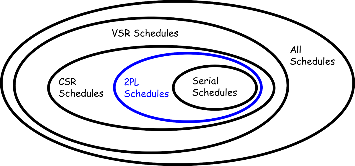
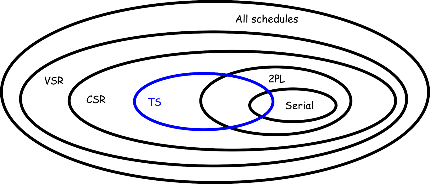
By adhering to this rule, 2PL guarantees that the resulting schedules are both view-serializable () and conflict-serializable (), ensuring a consistent and correct order of transaction operations.

2PL Implies CSR

The relationship between Two-Phase Locking (2PL) and Conflict-Serializability () can be summarized as follows:

Every 2PL schedule is also conflict-serializable

If a schedule follows the rules of 2PL, it cannot lead to a situation where conflicting operations are executed in a reverse order, which is a necessary condition for cycles in the precedence graph.

Proof

Assumption: Assume that a 2PL schedule is not conflict-serializable. This means the precedence graph of must contain at least one cycle, for example, .

Cycle Implication: For a cycle to exist, there must be a pair of conflicting operations that are executed in reverse order. We can denote the conflicting operations as follows:

: An operation by transaction .

: An operation by transaction .

: An operation by transaction on another data item .

: An operation by transaction on data item .

Locking Behavior:

For to access via , must have released the lock on (because of the two-phase rule).

If has released the lock, then can read or write to only if is not holding the lock anymore.

Contradiction:

Later in the schedule, for and to have conflicting operations on (i.e., and ), must have acquired the lock on .

Thus, the lock held by on implies that could not have released the lock on and still be conflicting with , which leads to a contradiction.

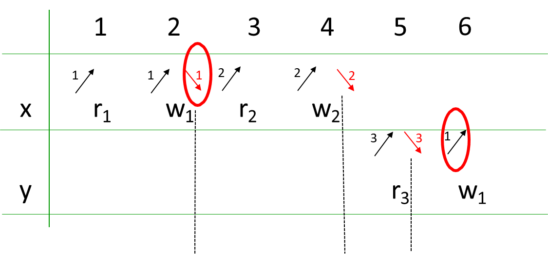
Conclusion: Hence, every 2PL schedule must be conflict-serializable, proving that .

While it is true that all 2PL schedules are conflict-serializable, the converse does not hold. That is, not every conflict-serializable schedule adheres to the 2PL rules.

Counter-Example
Consider the schedule:

This schedule can be interpreted as follows:

Transactions:

reads and writes .

reads and writes after has released the lock on .

reads and then writes to .

In this schedule:

releases the lock on after it has finished with its operations.

then proceeds to operate on , allowing to access between these operations.
graph LR
  T3 -- r3(y)w1(y) --> T1 -- r1(x)w2(x)<br>w1(x)w2(x) --> T2
This shows a scenario where:

Conflicting operations on are preserved in a serializable manner.

However, the lock management does not adhere to the two-phase rule as releases its lock and subsequently attempts to acquire another lock, thus violating 2PL.

2PL and Other Anomalies

While 2PL aims to ensure serializability and minimize anomalies, several issues can still arise, including:

Nonrepeatable read: A transaction reads a value, another transaction updates that value, and then the first transaction reads it again, resulting in different values.

Example: .

Lost update: Two transactions read the same value, but one transaction overwrites the changes of another, causing data loss.

Example: .

T1 releases a lock to T2 and then tries to acquire another one

Phantom update: Similar to lost updates, but concerning updates on records that were not originally present.

Example: .

T1 releases a lock to T2 and then tries to acquire another one

Phantom insert: A new record is inserted that matches a previous read operation after another transaction has released its locks.

Example:

This requires predicate locks to prevent future data from being inserted.

Dirty read: A transaction reads uncommitted changes made by another transaction, which can lead to inconsistencies.

Example:

This scenario needs to be addressed with strict locking protocols.

Strict Two-Phase Locking (Strict 2PL)

Strict Two-Phase Locking is a variation of the standard Two-Phase Locking protocol, designed to prevent anomalies associated with dirty reads and to ensure a higher level of isolation among transactions.

Lock Management: In strict 2PL, locks held by a transaction cannot be released until that transaction commits or rolls back. This ensures that once a transaction has acquired locks, it retains control over the data until it has definitively completed its operations.
Rollback Behavior: In the case of a rollback, the system restores the state of the database to the point prior to the aborted transaction’s updates, effectively preventing any dirty reads from occurring. This is crucial for maintaining data integrity and consistency.
Lock Duration: Strict 2PL locks are often referred to as long-duration locks, in contrast to standard 2PL locks, which are considered short-duration locks. This terminology reflects the fact that strict 2PL locks remain active until a transaction completes, as opposed to being released after individual operations within the transaction.
Implementation in Commercial DBMSs: Most commercial DBMS implement strict 2PL when a high level of isolation is required. This is especially important in systems where data consistency is critical, such as financial applications.
Variable Policies for Lock Types: Real systems may apply different policies for read and write locks under strict 2PL. For instance, while write locks may be held for the duration of the transaction, read locks might have more flexible handling, often implemented with less stringent conditions.
Performance Considerations: Long-duration read locks can be expensive in terms of system performance. As a result, real systems often utilize more sophisticated mechanisms to manage read locks efficiently, such as shared locks or versioning strategies.

Predicate Locks

To address the issue of phantom inserts, strict 2PL can utilize predicate locks. These locks extend the locking mechanism beyond simple data items to encompass future data that may satisfy a query.

Definition

A phantom insertion occurs when a new item is added to a dataset that was previously read by another transaction. This can create inconsistencies, as the new item might affect the outcome of queries executed by the first transaction.

To prevent phantom inserts, a lock should be placed on “future data”. This means that any transaction that could potentially affect the outcome of previous queries must be restricted from inserting or modifying relevant data.

Example
For example, consider a transaction that executes the operation:
UPDATE Tab SET b = 1 WHERE a > 1
In this case, the lock would apply to the predicate . Other transactions would then be prevented from inserting, deleting, or updating any tuple that satisfies this predicate.

If predicate locks are not supported by the implementation, the lock may need to extend to the entire table to cover all potential conflicts. However, if the system supports predicate locks, these can be managed using indexes and techniques like gap locking to optimize performance while maintaining data integrity.

The Impact of Locking

When transactions request locks, they are either granted the lock or suspended and queued in a first-in, first-out manner. This process carries the risk of deadlock and starvation.

Deadlock occurs when two or more transactions are in an endless mutual wait, typically happening when each transaction waits for another to release a lock.

For example, consider the sequence , where each transaction is waiting for the other to release a lock, leading to a deadlock situation.

Starvation, on the other hand, happens when a single transaction is in an endless wait. This typically occurs due to write transactions waiting for resources that are continuously being read, such as index roots. In such cases, the write transaction may never get the chance to acquire the necessary lock, leading to starvation.

Deadlocks

Definition

Deadlock in database management systems (DBMS) is a situation that arises when multiple concurrent transactions become locked in a cyclic waiting pattern, each holding resources that other transactions require and awaiting resources held by those transactions in return.

Example
Suppose transaction first holds a read lock on resource and requests a write lock on resource , while transaction holds a read lock on and requests a write lock on .

This mutual holding-and-waiting relationship causes a deadlock, as illustrated in a lock graph or wait-for graph, where cycles indicate deadlock situations.
graph LR
    T1 -- holds(SL) --> x[(x)]
    T2 -- holds(SL) --> y[(y)]

    T1 -. requests(XL) .-> y
    T2 -. requests(XL) .-> x

Lock Graph and Wait-for Graph

In order to analyze and detect deadlocks, two main types of graphs are used: the lock graph and the wait-for graph.

The lock graph is a bipartite representation, where the nodes represent either transactions or resources, and the arcs between them indicate lock requests or current lock assignments.

Example
For instance, in the graph representation of the previous example, holds a lock on but requires a lock on , while holds a lock on but requests . In this case, each transaction “holds” or “requests” different resources, forming a cycle that represents a deadlock.
graph LR
	x[(x)]
	y[(y)]
	
    T1 -- holds(XL) --> x -. requested-by (SL) .-> T4
    x -. requested-by (SL) .-> T2 -- holds(SL) --> y -. requested-by (XL) .-> T1
    T3 -- holds(SL) --> y

Alternatively, the wait-for graph focuses on relationships between transactions alone. Here, each node represents a transaction, and arcs denote “waits-for” relationships. A cycle in this graph directly represents a deadlock.

Example
For instance, if is waiting for to release a resource while is simultaneously waiting for , they form a cycle in the wait-for graph. Deadlocks become apparent when these cycles occur, and breaking the cycle involves terminating one or more transactions involved in the deadlock.
graph LR
    T4 -- waits-for --> T1 -- waits-for --> T2 -- waits-for --> T1 -- waits-for --> T3

Deadlock Resolution Techniques

To resolve deadlocks, various techniques can be applied, each with its own approach and trade-offs. The main techniques are timeout-based resolution, deadlock prevention, and deadlock detection.

Technique	Principle	Deadlock Potential	Transaction Abort Rate	Typical Use Case
Timeout	Abort after waiting too long	Possible	Medium	Simple systems, legacy DBMS
Deadlock Prevention	Avoid cycles via ordering/IDs	Prevented	High (if contention)	High-concurrency, critical apps
Deadlock Detection	Detect cycles, abort to resolve	Possible	Low/Medium	Distributed DBMS, large systems
Wait-Die / Wound-Wait	Age-based abort/wait strategies	Prevented	Medium	Systems needing fairness/efficiency

Timeout Method

In the timeout approach, a transaction that has been waiting beyond a certain threshold is assumed to be in a deadlock. The system terminates this transaction and restarts it. This method is simple and was widely used in early database systems due to its low complexity.

However, setting the timeout threshold can be challenging:

if the timeout is too long, transactions will remain blocked unnecessarily, leading to poor system performance.
If it is too short, transactions may be terminated prematurely, increasing system overhead and reducing efficiency.

Deadlock Prevention

Deadlock prevention involves designing a system that proactively prevents the formation of cycles in the wait-for graph, thereby avoiding deadlocks before they happen. Prevention methods are either resource-based or transaction-based.

Resource-based prevention imposes strict rules on how resources can be requested. Transactions must request all resources they need upfront in a single batch, and once they have acquired them, they cannot request additional resources. Alternatively, resources can be globally ordered, and transactions are required to request them in this global order. The drawback of this method is its impracticality, as transactions often cannot anticipate all resources they will need at the start.
Transaction-based prevention assigns unique identifiers (IDs) to transactions, based on attributes like their start time or other “age” characteristics. Two well-known techniques under transaction-based prevention are:
- Wound-Wait: If an older transaction requests a resource held by a younger one, it preempts the resource (forces the younger transaction to release it).
- Wait-Die: If a younger transaction requests a resource held by an older transaction, it is forced to wait, thus reducing the chances of deadlock.

While these strategies prevent deadlock formation, they may lead to high transaction termination rates, causing inefficiency when implemented in systems with high concurrent processing demands.

Wait-Die Algorithm

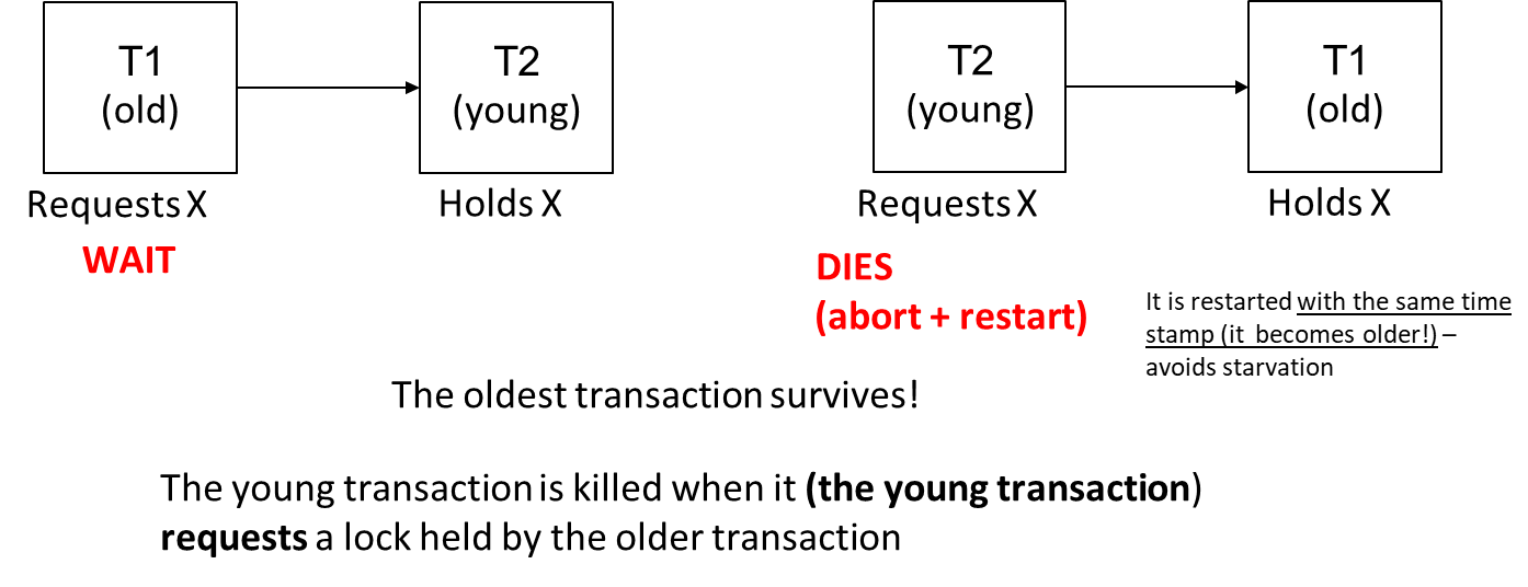
The Wait-Die algorithm is a non-preemptive conflict resolution method. In this algorithm, the outcome of a conflict between transactions is determined by their respective ages. Specifically,

if the requesting transaction is older than the conflicting transaction , then will wait for to release the lock. Conversely, if is younger than , "dies," meaning it is aborted and must be restarted.

Example

For example, consider the following scenario:

When (the older transaction) requests access to a resource already held by (the younger transaction), will wait until releases the lock.

However, if requests access to a resource held by , the younger transaction is aborted and restarted with the same timestamp, effectively making it “older.”

This mechanism prevents starvation, as can still be executed once it is restarted. The essence of the Wait-Die algorithm lies in its principle that the oldest transaction survives, thereby ensuring that resources are allocated based on transaction age.

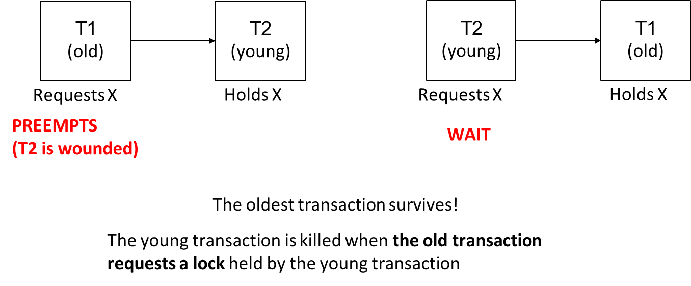
Wound-Wait Algorithm

In contrast, the Wound-Wait algorithm is a preemptive strategy. Similar to the Wait-Die algorithm, this algorithm also considers the ages of the transactions involved in a conflict.

If (the older transaction) requests a lock held by (the younger transaction), will "wound" . In this case, is aborted immediately, allowing to proceed with its operation. If is younger than , then will wait for to release the lock.

The dynamics of the Wound-Wait algorithm can be illustrated as follows:

Example

When (the older transaction) attempts to access a resource that (the younger transaction) holds, is aborted, and can continue.

On the other hand, if requests access to a resource held by , must wait.

This approach emphasizes the principle that the oldest transaction should prevail in accessing resources, thereby reinforcing efficient resource utilization and reducing the likelihood of deadlock situations.

Deadlock Detection

Deadlocks can occur in transaction management systems when two or more transactions are waiting for each other to release resources, resulting in a cycle of dependencies that cannot be resolved. Detecting such cycles, especially in distributed environments, is a complex challenge that requires a sophisticated algorithm. One notable solution is Obermarck’s algorithm, originally developed for IBM’s DB2 system and detailed in ACM Transactions on Database Systems.

To efficiently detect deadlocks in a distributed setting, the algorithm utilizes a representation of transaction status across various nodes.

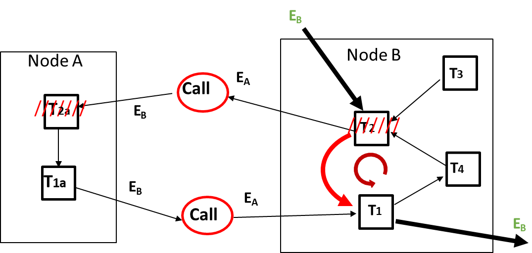
For instance, consider the following scenario involving two nodes, Node A and Node B:

At Node A, the wait-for relationships can be represented as:
At Node B, the relationships are:

In this notation, the symbol signifies a “wait-for” relationship among local transactions. If one term is an external call, it indicates that either the source is being waited for by a remote transaction or the sink is waiting for a remote transaction.

A potential deadlock occurs when there is a cycle in the wait-for graph, such as:

waits for (data lock)
waits for (external call)
waits for (data locks)
waits for (external call)

This situation forms a cycle that indicates a deadlock.

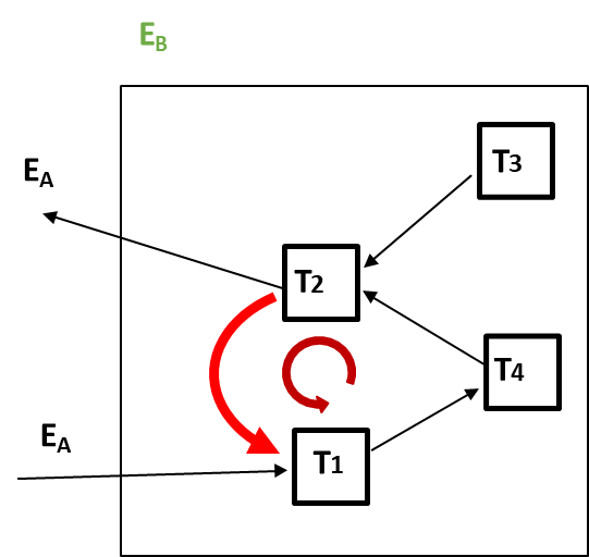
To illustrate this further, a distributed dependency graph can be created. External “call” nodes represent the interactions between sub-transactions across different nodes, enabling the visualization of dependencies and potential deadlocks. The graph can be depicted as follows:

graph LR
    subgraph "Node A"
      direction TB
      T2a --> T1a
    end

    subgraph "Node B"
      direction RL
        T3 --> T2b
        T1b --> T4 --> T2b
    end

    T2b -- EA --> Call1((Call)) -- EB --> T2a
    T1a -- EB --> Call2((Call)) -- EA --> T1b

In this graph, arrows represent the “wait-for” relationships among the transactions, with external calls indicating the interactions between transactions at different nodes. By analyzing this graph, the algorithm can detect cycles that signify deadlocks without maintaining a global view of the entire system.

Obermarck’s Algorithm

Obermarck’s Algorithm is a sophisticated method designed to detect potential deadlocks in a distributed system by analyzing the local view of each node involved.

The primary goal of this algorithm is to efficiently identify deadlock conditions without requiring a global view of all system transactions.

This is accomplished through the establishment of a communication protocol that allows each node to maintain a local projection of the global dependencies among transactions.

In practice, the algorithm facilitates the exchange of information between nodes, allowing them to update their local graphs based on the dependencies reported by other nodes. This information exchange is optimized to prevent multiple nodes from detecting the same potential deadlock simultaneously, which is crucial for maintaining system efficiency. The communication is governed by specific rules that dictate when one node should share its local transaction information with another.

For instance, a node A will transmit its information to node B only if it is waiting for a transaction, denoted as , from a remote source while simultaneously waiting for a transaction that is currently active on node B, with the condition that .

This condition ensures that messages are forwarded in a manner that reflects the order of transactions, creating a directed path of information flow. In simpler terms, node A only sends information to node B if it is waiting on a transaction listed at node B with a smaller index than its own.

graph LR
    subgraph "Node A"
      direction TB
      T2a --> T1a
    end

    subgraph "Node B"
      direction RL
        T3 --> T2b
        T1b --> T4 --> T2b
    end

    T2b -- EA --> Call1((Call)) -- EB --> T2a
    T1a -- EB --> Call2((Call)) -- EA --> T1b

The forwarding rule is illustrated through the following interactions between two nodes, A and B.

In this scenario, node A has an activation and waiting sequence represented as , where it is waiting for while being dependent on . The indices associated with these transactions are and . Since , node A is permitted to dispatch its information to node B.
Conversely, node B’s sequence indicates that it is waiting for transaction while being dependent on (with and ). Here, since , node B does not send any information back to node A.

Steps of Obermarck's Algorithm

Obermarck’s Algorithm runs periodically at each node and follows these four steps:

Gather Information: Each node collects wait dependencies and external call information from preceding nodes. This includes node and top-level transaction identifiers.

Update Local Graph: The node merges the new information with its existing data to update the local transaction graph.

Check for Cycles: The algorithm looks for cycles in the local graph, which indicate potential deadlocks. If a cycle is found, one transaction in the cycle is terminated to resolve the deadlock.

Send Updated Information: The node sends its updated graph information to the next nodes in the network.

In the initial phase of Obermarck’s Algorithm, the focus is on establishing communication between nodes to facilitate deadlock detection. This involves the application of a forwarding rule that governs when one node should send its information to another node in the network.

At Node A, the sequence of transactions is represented as . In this scenario, Node A has active dependencies where it is waiting for while simultaneously being dependent on . As a result, Node A sends its information to Node B because it satisfies the condition (where corresponds to and corresponds to ).
Conversely, at Node B, the sequence is structured as . Here, Node B is not in a position to send any information back to Node A since it does not meet the forwarding condition, specifically (where corresponds to and corresponds to ).

This selective communication helps to prevent unnecessary information exchange and optimizes the overall process.

In the second step of the algorithm, Node B updates its local wait-for graph based on the information it received from Node A. The process unfolds as follows:

Receiving Information: Node B receives the message from Node A.
Updating the Local Graph: The received sequence is integrated into Node B’s local wait-for graph. This update reflects the new dependencies introduced by the information from Node A.
Deadlock Detection: Upon updating the graph, Node B checks for cycles among the transactions. In this case, a cycle is identified involving and , indicating a potential deadlock condition. To resolve this deadlock, one of the transactions—either , , or another related transaction —must be terminated or rolled back to allow the other transactions to proceed.

Obermarck: Immateriality of Conventions

An interesting aspect of Obermarck’s Algorithm is its flexibility concerning certain arbitrary choices that can affect its implementation:

Forwarding Condition: The algorithm can operate with different forwarding conditions:

(1) Send messages only if

(2) Send messages only if

Message Destination: The algorithm also allows for variations in message destinations:

(a) Send messages to the following node

(b) Send messages to the preceding node

These choices give rise to four distinct versions or variants of the algorithm: (1+a), (1+b), (2+a), and (2+b). While the sequence of messages transmitted between nodes may differ among these variants, they share a common objective: effectively identifying deadlocks when they arise within the system. This adaptability highlights the robustness of Obermarck’s Algorithm, making it a valuable tool for managing distributed systems with dynamic transaction interactions.

Deadlocks in Practice

In the realm of database management, deadlocks, though less frequent than conflicts, remain a significant concern. The probability of encountering a deadlock is notably lower than that of a conflict, particularly in scenarios involving transactions accessing shared resources.

Example

For instance, consider a file containing records with two transactions each performing 2 accesses. The likelihood of a conflict occurring can be quantified as , derived from the summation:

In contrast, the probability of a deadlock emerges as . This is because a deadlock requires that Transaction 1 () conflicts with Transaction 2 () and vice versa, leading to a compounded probability that is quadratic in nature.

Despite this lower probability, deadlocks do occur with measurable frequency—on average, once every minute in a mid-sized bank. The likelihood of deadlocks tends to be linear concerning the number of concurrent transactions and quadratic relative to their lengths, as measured by the number of lock requests. Therefore, shorter transactions generally reduce the risk of deadlocks, given all else being equal.

Update Lock

A prevalent cause of deadlocks arises when two concurrent transactions begin by reading the same resource under Shared Locks () and later attempt to write to the resource, requiring an upgrade to Exclusive Locks (). This sequence creates a situation ripe for conflict. To mitigate this scenario, database systems employ the Update Lock (UL) mechanism.

An Update Lock is specifically designed for transactions that will read data and subsequently write to it. This type of lock serves to signal the intention of a transaction to modify a resource after initially reading it, thus preventing the deadlock condition described above.

Resource Status	Free	SL	UL	XL
SL	✔️	✔️	✔️	❌
UL	✔️	✔️	❌	❌
XL	✔️	❌	❌	❌

In this context, the status of the resource dictates the compatibility of various lock types. A Shared Lock () can coexist with other s and Update Locks (), while it cannot coexist with an Exclusive Lock (). An Update Lock () can be granted only if the resource is free or currently under an , whereas it cannot coexist with another or any . Exclusive Locks () are the most restrictive, allowing no other locks.

To request an Update Lock in practice, a transaction can use the SQL statement:

SELECT * FROM table_name FOR UPDATE;

This command effectively signals the database system to grant an Update Lock, enabling the transaction to read the data while preparing for a subsequent write operation. By implementing Update Locks, databases can significantly reduce the likelihood of deadlocks, leading to more efficient transaction management and enhanced system performance.

Hierarchical Locking

Hierarchical locking is a technique used in database management systems to control access to resources while minimizing contention among transactions. This approach employs a structured framework that allows for varying degrees of lock granularity, which in turn can optimize concurrency. The granularity of locks can be specified at different levels, including schema, table, fragment, page, tuple, and field. This flexibility allows transactions to lock only the necessary amount of data, thereby reducing the potential for conflicts and enhancing overall system performance.

One of the primary objectives of hierarchical locking is to lock the minimum amount of data required for a transaction to execute successfully. This is achieved by extending the locking interval judiciously, meaning that resources are held only as long as necessary. Consequently, it becomes critical to decide what to lock; for instance, locking an entire table might significantly reduce concurrency, which is undesirable in high-transaction environments. Thus, the locking mechanism should be carefully designed to recognize conflicts as early as possible, allowing for more efficient resource management.

The method employed in hierarchical locking involves a top-down approach for requesting locks on hierarchical resources. Transactions initiate requests from the root level—typically the entire table—and navigate down the hierarchy until they reach the appropriate level of granularity required for their operations. Conversely, locks are released in a bottom-up fashion, starting from the locked resource and proceeding up the hierarchy. This structured approach not only facilitates efficient resource usage but also helps maintain consistency within the database.

Intention Locking Scheme

The intention locking scheme enhances the hierarchical locking protocol by introducing additional lock modes beyond the traditional shared (SHARED) and exclusive (EXCLUSIVE) locks. These new modes express the “intention” of locking at lower levels of granularity, providing more nuanced control over resource access. The three additional modes include Intention Shared Lock (ISL), Intention Exclusive Lock (IXL), and Shared with Intention Exclusive Lock (SIXL).

The Intention Shared Lock (ISL) indicates that a transaction intends to acquire shared locks on sub-elements of the current resource.
The Intention Exclusive Lock (IXL) signals an intention to lock sub-elements in exclusive mode, preventing other transactions from acquiring either shared or exclusive locks on those sub-elements.
The Shared with Intention Exclusive Lock (SIXL) represents a combination where the parent resource is locked in shared mode while signaling the intention to lock a sub-element exclusively.

This intention-based approach improves the efficiency of the locking mechanism by providing a clear signal about a transaction’s future locking intentions, thereby allowing for better management of concurrent access.

Hierarchical Locking Protocol

The hierarchical locking protocol dictates how locks are requested and released within the system. When a transaction requests a lock, it starts from the root of the hierarchy (e.g., the entire table) and proceeds downward.

To successfully request an SL or ISL lock on a non-root element, the transaction must already hold an equally or more restrictive lock on its parent resource.
Similarly, to acquire an IXL, XL, or SIXL lock on a non-root element, the transaction must hold a more restrictive lock on its parent.

This requirement ensures that the locking hierarchy is respected and maintained throughout the transaction lifecycle.

The decision-making process for granting locks is managed by the lock manager, which refers to a predefined hierarchical lock granting table. The hierarchical lock granting table serves as a reference for lock compatibility, delineating which lock types can coexist.

An ISL request can be granted under any condition, including when the resource is free or already held by other ISL, IXL, SL, or SIXL locks. However, it cannot be granted if an XL lock is already held.
An IXL request is similarly flexible but will be denied if an SL or XL lock is present.
A SL request can coexist with other SL and ISL locks but will be denied if an XL or SIXL lock is held.
A SIXL request is more restrictive, permitting only ISL locks to coexist.
An XL request is the most restrictive, allowing no other locks on the resource.

Request	Free	ISL	IXL	SL	SIXL	XL
ISL	✔️	✔️	✔️	✔️	✔️	❌
IXL	✔️	✔️	✔️	❌	❌	❌
SL	✔️	✔️	❌	✔️	❌	❌
SIXL	✔️	✔️	❌	❌	❌	❌
XL	✔️	❌	❌	❌	❌	❌

Concurrency Control with Timestamps

Concurrency control using timestamps is an approach that allows databases to manage transactions efficiently while preserving consistency, without the need for traditional locking mechanisms. This method is based on timestamp ordering and is often referred to as an optimistic concurrency control technique. Unlike locking, which is also called pessimistic concurrency control, timestamp-based control operates under the assumption that transaction conflicts are relatively infrequent, and thus, transactions can be processed without locking resources in advance.

In pessimistic concurrency control, systems assume conflicts will occur between transactions attempting to access the same resource simultaneously, so they use locks to avoid inconsistencies. The assumption is that conflicts are common, so preventing transactions from conflicting is a priority. In contrast, optimistic concurrency control assumes that conflicts are rare; transactions are allowed to proceed without locks, and validation checks occur just before committing to ensure no conflicting changes were made. In timestamp-based control, timestamps are assigned to each transaction as a unique identifier to track the order of transactions and verify if conflicts occur.

Definition

A timestamp is an identifier assigned to each transaction when it begins, indicating the “birth time” of the transaction. This birth timestamp defines a total order of transactions and determines which transactions are “older” or “newer.”

This ordering is important because a schedule is only accepted if it reflects a serial ordering consistent with each transaction’s timestamp.

For example, in a timestamp-based concurrency control system, the system assigns an ascending numeric timestamp to each transaction. A lower timestamp value indicates an older transaction, which generally means it has higher priority to complete operations on shared resources compared to newer transactions with higher timestamps.

In a timestamp-based concurrency control system, two key counters are maintained for each object (e.g., a record in a database):

Read Timestamp (): This is the highest timestamp of any transaction that has successfully read the object .
Write Timestamp (): This is the highest timestamp of any transaction that has successfully written to the object .

When a transaction makes a request to read or write an object, these timestamps are referenced to determine whether the request can be granted. For each read or write request, the transaction’s timestamp is compared to and to check for potential conflicts.

Principles of Timestamp-Based Concurrency Control

Read Requests ():
- If the timestamp of the requesting transaction () is less than , this indicates that the transaction is trying to read a version of that has already been updated by a newer transaction. In this case, the read request is denied, and the transaction is terminated.
- Otherwise, if the timestamp is greater than or equal to , the read request is granted. The is then updated to the maximum of its current value and the transaction’s timestamp.
Write Requests ():
- If the transaction’s timestamp is less than , it means there is a conflict: an older read has already occurred that should precede this write, so the write request is rejected, and the transaction is terminated.
- Additionally, if the timestamp is less than , this indicates that the transaction is attempting to overwrite a newer value, and the request is again denied.
- If neither of these conditions hold, the write request is allowed, and is updated to the timestamp of the current transaction.

Example of Timestamp-Based Concurrency Control

Consider the following scenario: The system starts with RTM(x) = 7, indicating that the last read on object was performed by a transaction with timestamp 7, and WTM(x) = 4, meaning the last write was performed by a transaction with timestamp 4.

Request Response RTM(x) WTM(x)
7 4
r₆ (x) ✔️ (6>4)
r₈ (x) ✔️ (8>4) 8
r₉ (x) ✔️ (9>4) 9
w₈ (x) ❌ (8<9) T8 killed
w₁₁ (x) ✔️ (11>9 and 11>4) 11
r₁₀ (x) ❌ (10<11) T10 killed

For a series of requests:

Transaction with r6(x) (read by a transaction with timestamp 6):

Since 6 > WTM(x), the read request is allowed.

RTM(x) remains 7 because it is already higher than 6.

Transaction with r8(x) (read by a transaction with timestamp 8):

Since 8 > WTM(x), this read request is allowed, and RTM(x) is updated to 8.

Transaction with w8(x) (write by a transaction with timestamp 8):

Since 8 < RTM(x) (RTM(x) is now 9, indicating a more recent read), this write request is denied, and transaction T8 is terminated.

Transaction with w11(x) (write by a transaction with timestamp 11):

Both conditions are met (11 > RTM(x) and 11 > WTM(x)), so this write request is granted, and WTM(x) is updated to 11.

Transaction with r10(x) (read by a transaction with timestamp 10):

Since 10 < WTM(x), this request is denied, and transaction T10 is terminated.

Request	Response	RTM(x)	WTM(x)
		7	4
r₆ (x)	✔️ (6>4)
r₈ (x)	✔️ (8>4)	8
r₉ (x)	✔️ (9>4)	9
w₈ (x)	❌ (8<9)			T8 killed
w₁₁ (x)	✔️ (11>9 and 11>4)		11
r₁₀ (x)	❌ (10<11)			T10 killed

Comparison Between Two-Phase Locking (2PL) and Timestamp-Based Concurrency Control (TS)

Two-Phase Locking (2PL) and Timestamp-based concurrency control (TS) represent two fundamental approaches to managing concurrent transactions in databases. While both techniques aim to preserve transaction consistency, they operate on distinct principles and are not always directly comparable due to differences in their behavior and constraints.

Two-Phase Locking (2PL) uses a locking mechanism to enforce a serialization order based on transaction conflicts. In 2PL, a transaction has two phases: the “growing phase,” where locks are acquired, and the “shrinking phase,” where locks are released. A transaction cannot acquire new locks after it starts releasing them. This method ensures consistency by actively managing locks, which may lead to waiting and, in some cases, deadlocks. However, it achieves strict serialization by waiting for other transactions to release resources, so conflicts are managed in real-time through locks.
Timestamp-Based Concurrency Control (TS), on the other hand, orders transactions using timestamps assigned at the start of each transaction. Each transaction carries a unique timestamp that dictates its execution priority; older transactions (lower timestamps) have precedence. Instead of waiting for resources to be freed, TS kills transactions that violate the timestamp order, restarting them with new timestamps if necessary. This approach is optimistic, assuming conflicts are infrequent and avoiding locking delays. While it prevents deadlocks, it may incur a higher rate of transaction restarts, as conflicting transactions are terminated rather than queued.

Because 2PL and TS operate on different principles, there are cases where a schedule (or sequence of operations) can be valid in one but not in the other. For instance:

Schedule in TS but not in 2PL: If a transaction reads or writes in a sequence that violates 2PL’s locking constraints but preserves TS ordering by timestamps.

Example: r1(x) w1(x) r2(x) w2(x) r0(y) w1(y)
Schedule in 2PL but not in TS: If a schedule conforms to 2PL’s locking sequence but does not satisfy TS’s timestamp ordering.

Example: r2(x) w2(x) r1(x) w1(x)
Schedule both in TS and 2PL: A sequence that meets the requirements of both TS and 2PL while also maintaining a non-serial order.

Example: r1(x) r2(y) w2(y) w1(x) r2(x) w2(x)

Certain schedules may be serializable under TS but fail under 2PL constraints due to the differences in conflict management and locking.

Key Differences Between 2PL and TS

Active Waiting vs. Transaction Restarting: In 2PL, transactions may actively wait for resources if a conflict occurs, whereas in TS, conflicting transactions are terminated and restarted, which can increase overhead when conflicts are frequent.

Serialization Order: In 2PL, the serialization order is determined by the actual conflicts and lock acquisitions, while in TS, it is imposed by the predetermined timestamp ordering.

Deadlock Potential: 2PL can lead to deadlocks, especially in systems with high contention. TS, by contrast, prevents deadlocks by aborting conflicting transactions rather than queuing them, thus avoiding cyclic waits.

Delay and Restart Costs: Restarting transactions can be more costly than waiting for locks to be released in 2PL, especially in high-contention environments where frequent restarts reduce system throughput.

Practical Implementation: Many commercial databases implement a blend of both approaches, combining strict 2PL for essential locks with multi-version or TS-based techniques to enhance flexibility and performance. For example, systems may use Strict 2PL along with a Multi-Version Timestamp Ordering (MVTO) for greater concurrency.

Timestamp-Based Concurrency Control and Conflict-Serializable Reads (CSR)

In TS, schedules can be Conflict Serializable () because of the inherent ordering imposed by timestamps. When TS is applied to a schedule, it ensures that all operations reflect the serial order defined by the timestamps, effectively preventing cycles (or circular dependencies) between transactions. For instance, if a cycle were to occur, it would imply that one transaction has read or written a value that contradicts the timestamp order, leading to the immediate termination of the conflicting transaction. This mechanism helps maintain CSR by terminating transactions that could otherwise introduce conflicts.

Example

For example, suppose TS enforces a schedule between transactions and where starts before and has a lower timestamp. If attempts to access a value already read or written by , TS will terminate , preserving the CSR by preventing a conflicting cycle.

TS Control and Dirty Reads

TS-based control generally considers only committed transactions, operating under a “commit-projection hypothesis” that ignores any aborted transactions in the scheduling order. This assumption helps simplify TS’s operation. However, it can lead to dirty reads if transactions are allowed to read data written by transactions that may eventually abort.

To prevent dirty reads, a modified TS approach can delay read operations until the committing or aborting status of the writing transaction is confirmed. In practice, this approach can add latency but helps ensure that only committed data is accessed.

For example, if writes to but has not yet committed, and (a newer transaction) attempts to read , TS may delay ’s read until either commits or aborts, thus ensuring that only reads stable, committed data.

Reducing the Kill Rate: Thomas’s Write Rule

To reduce the high transaction restart rate in TS, the Thomas Write Rule offers a strategy that minimizes unnecessary aborts.

Thomas's Write Rule

In TS, the system maintains two counters, and , to track the most recent read and write timestamps for each object . When a transaction requests to write to , TS checks the timestamp conditions:

If , the write is rejected because is trying to overwrite a value that has already been read by a more recent transaction, resulting in ‘s termination.

If , the write is deemed obsolete since a newer transaction has already written to . However, rather than killing , the Thomas Rule allows the system to skip this obsolete write without affecting consistency.

Otherwise, the write is accepted, and is updated to the timestamp of .

The Thomas Write Rule permits skipping outdated writes, which reduces transaction termination rates and improves throughput. However, this rule only applies if the write operation is independent of previous reads on the object; for instance, operations like SET X = X + 1 cannot skip writes without risking incorrect results.

Multiversion Concurrency Control (MVCC)

Multiversion Concurrency Control (MVCC) is a method for handling concurrent transactions by maintaining multiple versions of data items. This approach allows multiple transactions to access different versions of the same data item simultaneously, thereby improving concurrency.

The core idea of MVCC is to create new versions of data objects upon each write, rather than overwriting existing data, allowing reads to access the "right" version based on the timestamp of each transaction.

Version Creation: Every write operation generates a new version of a data item instead of replacing the existing value. Each version is tagged with a unique timestamp, known as the Write Timestamp (), which marks the time of creation. This ensures that each data object has at least one active version, though there could be multiple versions based on the number of writes performed on it.
Version Management: The system maintains a unique global Read Timestamp () for each object , representing the timestamp of the most recent transaction that has successfully read . Multiple versions of are stored in a sorted manner, with the oldest version (smallest ) at the beginning and the latest version (largest WTM) at the end.
Garbage Collection: Older versions of data objects are discarded when there are no active transactions that need to access them. This process minimizes storage overhead and ensures that the system does not retain unnecessary versions.

Example of MVCC in Theory: TS-Multi Allowing Unordered Writes

Theoretical implementations of TS-Multi allow for unordered writes under specific conditions. Here’s how this works:

Read Requests: A read request, denoted as , is always accepted, with the system selecting the version of that aligns with the transaction timestamp . For instance:

If (the most recent version), the read will use the latest version.

Otherwise, the read will access an older version where .

Write Requests: A write request, denoted as , follows different rules:

If , the write is rejected, as this would violate timestamp order and cause conflicts.

If the write is accepted, a new version is created with the current timestamp , and (the number of versions) is incremented accordingly. Each version is kept in order from the oldest to the newest.

Consider an example where RTM(x) = 7, N = 1, and WTM_1(x) = 4. We observe the following behaviors:

Request Response RTM(x) WTM(x)
r₆ (x) ✔️ 7 WTM_1(x) = 4, N=1
r₈ (x) ✔️ 8
r₉ (x) ✔️ 9
w₈ (x) ❌ - T8 killed
w₁₁ (x) ✔️ WTM_2(x) = 11, N=2
r₁₀ (x) ✔️ on x1 10
r₁₂ (x) ✔️ on x2 12
w₁₄ (x) ✔️ WTM_3(x) = 14, N=3
w₁₃ (x) ✔️ WTM_3(x) = 13, WTM_4(x) = 14, N=4

In this example, the MVCC mechanism ensures that each read accesses the appropriate version, while each write operation creates a new version with a unique timestamp, allowing concurrent transactions to coexist without conflicts.

Request	Response	RTM(x)	WTM(x)
r₆ (x)	✔️	7	WTM_1(x) = 4, N=1
r₈ (x)	✔️	8
r₉ (x)	✔️	9
w₈ (x)	❌ - T8 killed
w₁₁ (x)	✔️		WTM_2(x) = 11, N=2
r₁₀ (x)	✔️ on x1	10
r₁₂ (x)	✔️ on x2	12
w₁₄ (x)	✔️		WTM_3(x) = 14, N=3
w₁₃ (x)	✔️		WTM_3(x) = 13, WTM_4(x) = 14, N=4

In real-world implementations, a more restricted version of TS-Multi under Snapshot Isolation (SI) is used to prevent issues like conflicts and ensure consistency. Here’s how the SI-based MVCC differs:

Read Requests (): The read process is identical to the theoretical version, where a copy of is selected based on the timestamp:
- If , the latest version is accessed.
- Otherwise, an appropriate older version is chosen, ensuring that each transaction views a consistent snapshot of the database.
Write Requests ():
- If or , the write request is rejected to avoid conflicts.
- If the write is accepted, a new version is created with as its timestamp, and is incremented.

Snapshot Isolation ensures that each transaction reads from a consistent snapshot taken at its start time, meaning that each transaction works on its private view of the database without interfering with other concurrent transactions.

TS-Multi Under Snapshot Isolation

Given RTM(x) = 7, N = 1, and WTM_1(x) = 4, consider these transactions:

Request Response RTM(x) WTM(x)
r₆ (x) ✔️ 7 WTM_1(x) = 4, N=1
r₈ (x) ✔️ 8
r₉ (x) ✔️ 9
w₈ (x) ❌ - T8 killed
w₁₁ (x) ✔️ WTM_2(x) = 11, N=2
r₁₀ (x) ✔️ on x1 10
r₁₂ (x) ✔️ on x2 12
w₁₄ (x) ✔️ WTM_3(x) = 14, N=3
w₁₃ (x) ❌ - T13 killed

In this practical scenario, transactions are managed in such a way that conflicting writes are rejected immediately to prevent inconsistent states, while non-conflicting reads and writes proceed smoothly.

Request	Response	RTM(x)	WTM(x)
r₆ (x)	✔️	7	WTM_1(x) = 4, N=1
r₈ (x)	✔️	8
r₉ (x)	✔️	9
w₈ (x)	❌ - T8 killed
w₁₁ (x)	✔️		WTM_2(x) = 11, N=2
r₁₀ (x)	✔️ on x1	10
r₁₂ (x)	✔️ on x2	12
w₁₄ (x)	✔️		WTM_3(x) = 14, N=3
w₁₃ (x)	❌ - T13 killed

Snapshot Isolation (SI)

Definition

Snapshot Isolation (SI) is an isolation level in database management systems that leverages multi-version concurrency control (MVCC). SI allows each transaction to operate on a “snapshot” of the data as it existed at the transaction’s start time, preventing it from seeing updates made by other concurrent transactions.

This method provides a balance between consistency and concurrency, especially suited for systems where read-heavy workloads are prevalent.

Key points about SI:

Transaction Start Snapshot: Every transaction in SI sees a consistent snapshot of the database as it existed at the start time, meaning it reads only the versions of data items that were committed before the transaction began.
Write Conflicts: Writes are deferred until the end of a transaction. If two concurrent transactions attempt to write to the same data item after taking snapshots, one of them will be aborted to prevent conflicts.
Optimistic Concurrency: SI is considered a form of optimistic concurrency control, as it assumes that conflicts between transactions are rare and only checks for conflicts at commit time.

Popular DBMSs that support Snapshot Isolation include Oracle, MySQL, PostgreSQL, MongoDB, and Microsoft SQL Server.

Write Skew

Although SI prevents many types of anomalies, it does not guarantee serializability, meaning it can allow certain non-serializable outcomes. One such anomaly is write skew:

Consider two concurrent transactions:

: UPDATE Balls SET Color=White WHERE Color=Black
: UPDATE Balls SET Color=Black WHERE Color=White

If executed in a serializable manner, the final state would have all balls either white or black, depending on the execution order.

SI allows both transactions to start with the same snapshot, leading them to read and then update data independently. The result is a configuration where black and white balls are swapped rather than unified under a single color, leading to the write skew anomaly.

This non-serializable outcome under SI results from the fact that SI allows concurrent transactions to modify data based on outdated snapshots, as long as the modifications don’t directly conflict in their writes.

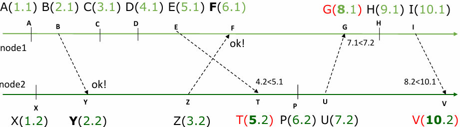
Timestamp Assignment in Distributed Systems

Assigning timestamps consistently in a distributed system without a global clock is challenging. In distributed databases, timestamps help order transactions and events across nodes.

Key points in timestamp management:

Timestamp Structure: Timestamps typically have the format event-id.node-id, where event-id is unique within each node.
Logical Ordering: Timestamps are treated lexically. For example, 5.1 (event 5 on node 1) is considered to happen before 5.2 (event 5 on node 2).
Synchronization via Messages: Using a messaging protocol, send-receive pairs are timestamped to maintain a causal order. The Lamport Logical Clock algorithm ensures that events are ordered logically even if they lack real-time synchronization.
Bumping Rule: If a node receives a message with a timestamp later than its own last timestamp, it increments (or “bumps”) its timestamp to align with the received message.

Example Scenario for Timestamp Assignment

Consider events occurring on different nodes:

Event Y and Event F: These represent messages received from the present or past, so timestamps align without adjustment.

Event T, G, and V: These represent messages from the “future.” In this case, each receiving node must bump its timestamp beyond the sender’s timestamp to maintain order. For instance, if G(8.1) represents event G from node 1 and U(7.2) was the previous event, G(8.1) bumps to 8.1 to maintain causal order.

Concurrency Control in Commercial DBMSs

Different commercial database systems implement SI and other concurrency control techniques with unique specifications:

Oracle: Uses multi-version concurrency control, enabling SI through “read consistency,” which maintains snapshots for each transaction. Oracle Documentation
MySQL: Implements SI in InnoDB through MVCC, using rollback segments to store previous versions of data rows. MySQL Documentation
IBM DB2: Uses a mix of pessimistic and optimistic concurrency control techniques and provides fine-grained isolation levels. DB2 Documentation
MongoDB: Uses a multi-version model for concurrency control. Write operations are isolated on a per-document basis, preventing read-write conflicts. MongoDB Documentation

Polimi CS - Notes

Explorer

4.3 - Concurrency Control in Practice and Locking

Table of Contents

Concurrency Control Approaches

Locking Mechanism in Concurrency Control

Two-Phase Locking (2PL)

2PL Implies CSR

2PL and Other Anomalies

Strict Two-Phase Locking (Strict 2PL)

Predicate Locks

The Impact of Locking

Deadlocks

Lock Graph and Wait-for Graph

Deadlock Resolution Techniques

Timeout Method

Deadlock Prevention

Wait-Die Algorithm

Wound-Wait Algorithm

Deadlock Detection

Obermarck’s Algorithm

Deadlocks in Practice

Update Lock

Hierarchical Locking

Intention Locking Scheme

Hierarchical Locking Protocol

Concurrency Control with Timestamps

Principles of Timestamp-Based Concurrency Control

Comparison Between Two-Phase Locking (2PL) and Timestamp-Based Concurrency Control (TS)

Timestamp-Based Concurrency Control and Conflict-Serializable Reads (CSR)

TS Control and Dirty Reads

Reducing the Kill Rate: Thomas’s Write Rule

Multiversion Concurrency Control (MVCC)

Snapshot Isolation (SI)

Write Skew

Timestamp Assignment in Distributed Systems

Concurrency Control in Commercial DBMSs

Backlinks

Graph View

Table of Contents