Supervised Learning for Fraud Detection

Supervised Learning relies on historical labeled data to identify known fraudulent patterns and build an analytical model for predicting a target measure of interest. The target is used to guide the learning process and determine whether a transaction is fraudulent or not. However, obtaining and determining the target fraud indicator can be challenging, and the labels may not be completely accurate. It is important to avoid overfitting in this complex analytical modeling exercise.

In Supervised Learning, the target measure can be continuous in regression tasks or categorical in classification tasks. Regression deals with variables that vary along a predefined interval, while classification is limited to a set of predefined values, such as binary or multiclass classification.

Linear Regression

Linear regression is a fundamental and widely used statistical technique in predictive modeling, particularly for analyzing and predicting continuous outcomes. It models the relationship between a dependent variable (or target variable) and one or more independent variables (also known as explanatory variables). The core idea behind linear regression is to fit a linear equation to observed data in such a way that the sum of the squared differences between the observed values and the predicted values is minimized.

The general linear regression model can be mathematically represented as:

where:

• is the target variable (the outcome we want to predict).
• are the independent variables (the predictors or features).
• is the intercept of the model, representing the expected value of when all independent variables are zero.
• are the coefficients (or parameters) corresponding to each independent variable. These coefficients quantify the impact of each independent variable on the target variable.

The linear regression model assumes a linear relationship between the independent variables and the dependent variable, meaning that changes in the independent variables result in proportional changes in the dependent variable.

The primary goal of linear regression is to estimate the parameters such that the model accurately predicts the target variable . This is achieved by minimizing the sum of squared errors (SSE), which is the sum of the squared differences between the observed target values and the predicted values :

Observation			…
1
2
…

where:

• is the actual target value for observation .
• is the predicted value for observation generated by the linear regression model.

Minimizing this sum of squared errors ensures that the model’s predictions are as close as possible to the actual observed values.

The most common method for estimating the parameters in a linear regression model is the Ordinary Least Squares (OLS) method. OLS aims to find the parameter values that minimize the sum of squared errors. The estimated parameters can be calculated using the following matrix equation:

In this equation:

• is the matrix of independent variables, where each row represents an observation and each column represents an independent variable. An additional column of s is included to account for the intercept term .
• is the vector of observed target values.
• is the vector of estimated coefficients.

The term is derived from setting the gradient of the sum of squared errors with respect to the parameters to zero and solving for .

NOTE

Linear regression relies on several key assumptions to produce valid results:

1. Linearity: The relationship between the independent and dependent variables is linear.
2. Independence: The observations are independent of each other.
3. Homoscedasticity: The variance of the errors is constant across all levels of the independent variables.
4. Normality of Errors: The errors (residuals) are normally distributed.

Violations of these assumptions can lead to biased or inefficient estimates, affecting the model’s predictive performance.

Linear regression is extensively used across various fields due to its simplicity and interpretability:

• Economics: For modeling and forecasting economic indicators like GDP, inflation, or unemployment rates.
• Finance: For assessing the relationship between asset prices and economic factors or predicting stock returns.
• Social Sciences: For understanding the impact of various social factors on outcomes like education, employment, or income.

Logistic Regression

Logistic Regression is a widely used statistical model for predicting the probability of a binary outcome (such as yes/no, success/failure) based on one or more independent variables. This method is particularly useful in situations where the response variable is categorical and needs to be constrained within the range of and , representing probabilities.

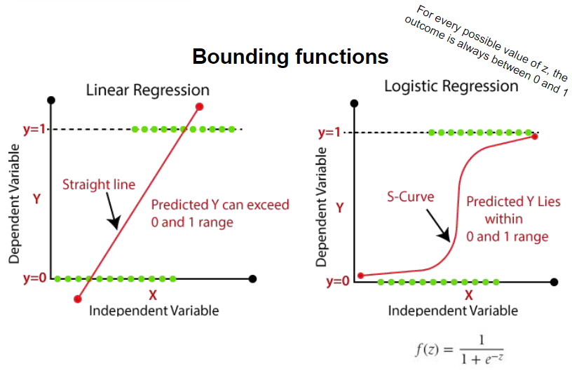
When attempting to model a binary outcome using Ordinary Least Squares (OLS), two significant challenges arise:

1. Non-Normal Distribution of Errors: OLS assumes that the errors (or residuals) follow a normal distribution. However, in the case of binary outcomes, the errors are distributed according to a Bernoulli distribution, which only takes on two possible values (typically and ). This violates the OLS assumption of normally distributed errors, making it inappropriate for binary classification tasks.
2. Unbounded Predictions: OLS does not inherently constrain the predicted values to the range of and . This can lead to predictions outside the probability range, which is not meaningful when predicting probabilities. Logistic Regression addresses this issue by ensuring that the predicted outcomes are always within the to range.

Definition

Logistic Regression is a statistical technique used primarily for binary classification tasks. It estimates the probability that a given input belongs to a particular class (e.g., success or failure). The model combines linear regression with a bounding function to ensure that the output remains within the range of 0 and 1, making it suitable for probability prediction.

Maximum Likelihood Estimation (MLE): The parameters () of a Logistic Regression model are estimated using Maximum Likelihood Estimation. MLE is a method that identifies the parameter values that maximize the likelihood of observing the given data. In the context of Logistic Regression, this involves finding the parameter values that best explain the observed binary outcomes.

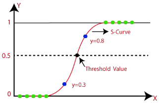
Sigmoid Activation Function: A key component of Logistic Regression is the sigmoid function, a type of activation function that maps the linear combination of input features (the weighted sum) to a value between and . The sigmoid function produces an S-shaped curve, which helps in converting the linear output of the model into a probability. The function is defined as: where is the linear combination of the input features and their corresponding weights.

Variable selection is a crucial step in building an effective Logistic Regression model. Choosing the right variables (or predictors) can significantly impact the model’s performance. Several methods are available for variable selection:

1. Forward Selection: Starts with no predictors in the model and adds them one by one, selecting the predictor that most improves the model at each step.
2. Backward Elimination: Starts with all potential predictors and removes them one by one, eliminating the predictor that has the least impact on the model at each step.
3. Stepwise Selection: Combines forward selection and backward elimination, allowing for both adding and removing predictors based on their statistical significance and contribution to the model.

When selecting variables, it is important to consider multiple criteria:

• Statistical Significance (p-value): The p-value helps assess the significance of each variable. A low p-value (typically less than ) suggests that the variable has a significant impact on the response variable, meaning it contributes meaningfully to the model’s predictions.
• Interpretability: The sign of the regression coefficient () indicates the direction of the relationship between a predictor and the response variable. A positive coefficient suggests that an increase in the predictor value leads to an increase in the predicted probability, whereas a negative coefficient suggests the opposite.
• Operational Efficiency: The practicality of including a variable in the model should be evaluated based on the resources required to collect and preprocess it. Variables that are expensive or time-consuming to obtain may not be ideal, especially in large-scale applications.
• Legal and Ethical Considerations: Some variables may be legally restricted or ethically inappropriate to use, such as those related to personal attributes (e.g., race, gender) that could lead to biased or discriminatory outcomes. It’s essential to ensure that the selected variables comply with legal guidelines and ethical standards.

Linear regression	Logistic regression
Prediction the continous dependent variable with indipendent variables	Predict the cetegorical dependent variable with indipendent variables
Find the best fit line/linear relationship (predict the output for the continous dependent variable based on indipendent variable)	Estimates a linear decision boundary to separate both classes
Ordinary least squares	Maximum Likelihood estimation
Regression (output: continuous values)	Classification (output: between 0 and 1)
	Regression

Decision Trees

Recursive-partitioning algorithms (RPAs) are used to create a tree-like structure that identifies patterns in a given dataset. The top node, known as the root node, represents a testing condition. The outcome of this condition determines which branch to follow, leading to an internal node. The terminal nodes, also known as leaf nodes, assign fraud labels.

The splitting decision in RPAs involves determining which variable to split and at what value. For example, a splitting decision could be based on whether the transaction amount is greater than $100,000 or not. The stopping decision determines when to stop adding nodes to the tree. Finally, the assignment decision involves assigning a class (e.g., fraud or no fraud) to a leaf node. This decision is typically made by considering the majority class within the leaf node, using a winner-take-all learning approach.

In some cases, each node in the tree may have only two branches, allowing the testing condition to be implemented as a simple yes/no question. However, in other cases, there may be more than two branches, resulting in multiway splits and wider but less deep trees.

It is worth nothing that every tree can also be represented as a rule set. Each path from the root node to a leaf node forms a simple if-then rule, which can be used to interpret the decision-making process of the tree.

Rule Set example

• if transaction amount > $100000 and unemployed = no then no fraud
• if transaction amount > $100000 and unemployed = yes then fraud
• if transaction amount < $100000 and previous fraud = no then no fraud
• if transaction amount < $100000 and previous fraud = yes then fraud

graph TD
    A[Transaction amount > $100,000]
    B[Previous fraud]
    C[Unemployed]
    D[Fraud]
    E[No fraud]
    F[Fraud]
    G[No fraud]

    A -- No --> B -- Yes --> D
    B -- No --> E
    A -- Yes --> C -- Yes --> F
    C -- No --> G

Splitting decision

To determine the splitting decision, it is important to understand the concept of impurity or chaos. Minimal impurity occurs when all customers are either classified as good or bad, while maximal impurity occurs when there is an equal number of good and bad customers.

There are two commonly used impurity measures:

• Entropy: It is calculated using the formula , where represents the probability of a customer belonging to class .
• Gini index: It is calculated as , where represents the probability of a customer belonging to class .

The goal of decision trees is to minimize the impurity in the data.

Candidate splits are evaluated based on their decrease in impurity, also known as the gain. A higher gain is preferred. The decision tree algorithm considers different candidate splits for each node, using a greedy and recursive strategy to select the split with the highest gain. This approach allows for parallelization and increases the efficiency of both sides of the tree.

Stopping decision

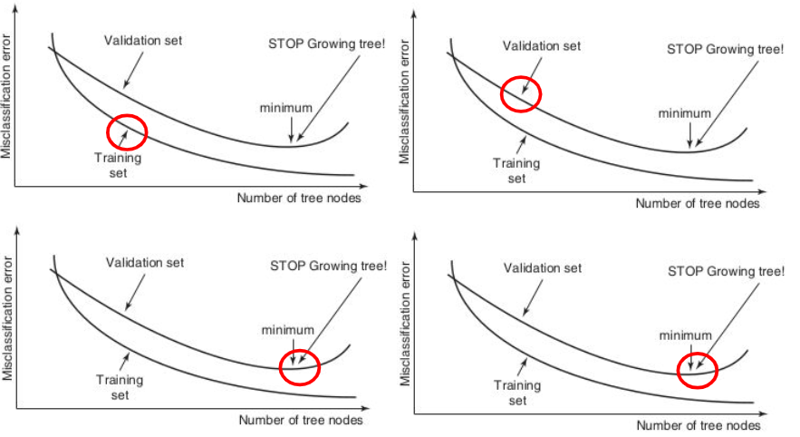
If the tree continues to split, it can result in one leaf node per observation, leading to overfitting. Overfitting occurs when the tree becomes too complex and fails to accurately capture the underlying trend in the data. This can cause poor generalization to new, unseen data. To avoid overfitting, it is recommended to split the data into a training sample (70%) for making splitting decisions and a validation sample (30%) for independently monitoring the misclassification error or other performance metrics.

During the training process, the error on the training sample may continue to decrease as the tree becomes more specific and tailored to the training data. However, on the validation sample, the error may initially decrease, indicating good generalization. But at some point, the error on the validation sample may start to increase as the tree becomes too specific to the training data, resulting in overfitting. It is important to stop the tree-building procedure when the validation error reaches its minimum to prevent overfitting.

Using decision trees in fraud analytics

Decision trees are a valuable tool in fraud analytics due to their ability to identify important variables and measure their predictive strength. The top variables in the tree are considered more predictive, and their gain is calculated to assess their power in predicting fraud. This analytical fraud model can be directly implemented in a business environment, providing clear explanations and interpretability.

Advantages:

• Interpretable: Decision trees are white-box models that offer a clear explanation of the decision-making process.
• Operationally efficient: They are efficient in terms of computational resources and can handle large datasets.
• Powerful techniques: Decision trees can capture complex decision boundaries, allowing for more accurate fraud detection than logistic regression.
• Non-parametric: Decision trees do not rely on assumptions of normality or independence.

Disadvantages:

• Sample dependency: Decision trees are highly sensitive to the sample used for construction. A slight variation in the sample can result in a completely different tree structure.

When using decision trees in fraud analytics, it is important to consider these advantages and disadvantages to make informed decisions and ensure accurate fraud detection.

Neural Networks

Quote

Neural networks are mathematical representations inspired by the functioning of the human brain

Neural networks can model very complex patterns and decision boundaries in the data.

Generalization of existing statistical models

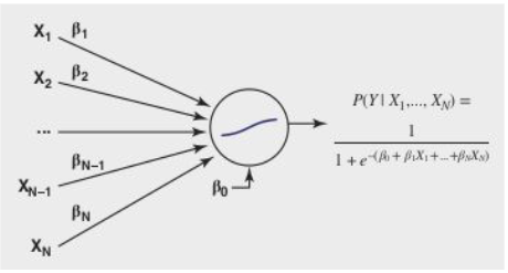
Logistic Regression is a widely used statistical model for binary classification. It estimates the probability of an event occurring based on a set of input variables. The logistic regression equation is defined as:

Interestingly, logistic regression can be viewed as a neural network with a single neuron and a sigmoid activation function. The neuron performs two operations: it takes the inputs and multiplies them with the corresponding weights (including the intercept term), and then applies a nonlinear transformation using the sigmoid function.

Neural networks, on the other hand, are more complex models that consist of multiple layers of interconnected neurons. They are capable of learning complex patterns and decision boundaries in the data. In a neural network, the input layer receives the input variables, the hidden layer(s) extract features from the inputs, and the output layer makes the final prediction.

Each neuron in a neural network applies an activation function to the weighted sum of its inputs. The choice of activation function depends on the layer and the task at hand. In the output layer, a logistic transformation is commonly used for classification tasks, as it produces probabilities. For regression tasks, different transformation functions can be used. In the hidden layer, a hyperbolic tangent activation function is often employed.

• Logistic activation function ranging between and
• Hyperbolic tangent: ranging between and
• Linear activation function: ranging between and

In the context of fraud analytics, where complex patterns are rare, it is recommended to use a neural network with a single hidden layer. These networks are known as universal approximators, as they can approximate any function with a desired level of accuracy within a compact interval. Before feeding the data into the neural network, it is important to preprocess the variables. Continuous variables should be standardized to ensure they have similar scales, while categorical variables can be categorized to reduce the number of categories.

By leveraging the power of neural networks and properly preprocessing the data, fraud analysts can build accurate and robust models for fraud detection and prevention.

Weight Learning

The process of optimizing parameter values for neural networks is a complex task that involves an iterative algorithm to minimize a cost function. The specific cost function used depends on the type of target variable being predicted. For continuous target variables, the Mean Squared Error (MSE) cost function is commonly used, while for binary target variables, the Maximum Likelihood cost function is preferred.

The optimization procedure starts with a set of random weights, which are then adjusted iteratively based on the patterns observed in the data. This adjustment is done using an optimization algorithm such as Backpropagation learning or Conjugate gradient. However, a key challenge in this process is that the objective function is not convex and may have multiple local minima. Therefore, it is crucial to choose the initial weights carefully to avoid getting stuck in suboptimal solutions.

To address this issue, a preliminary training phase can be conducted where different starting weights are tried out. The optimization procedure is then initiated for a few steps, and the best intermediate solution is selected to continue the training. The stopping criterion for the optimization procedure can be based on various factors, such as the lack of further progress in the error function, minimal changes in the weights, or a fixed number of optimization steps (epochs).

The number of hidden neurons in a neural network plays a crucial role in capturing the nonlinearity present in the data. Generally, more complex and nonlinear patterns require a larger number of hidden neurons. To determine the optimal number of hidden neurons, the data is typically split into a training set, a validation set, and a test set. The neural network is trained on the training set, and its performance is measured on the validation set. By varying the number of hidden neurons and evaluating the validation set performance, the number of hidden neurons that yield the best performance can be selected. Finally, the performance of the chosen neural network is measured on the independent test set to assess its generalization capability.

Overall, optimizing parameter values and determining the appropriate number of hidden neurons are crucial steps in building accurate and robust neural network models for various prediction tasks.

Overfitting Problem

Neural networks have the ability to capture complex patterns and decision boundaries in the data, including the noise present in the training data. There are two options to address the overfitting problem:

1. Option one: Use a validation set, which is an independent data set used to determine when to stop training and prevent overfitting. The weights are estimated using the training set.
2. Option two: Implement weight regularization, which involves keeping the weights small in absolute terms to prevent fitting the noise in the data. This is achieved by adding a weight size term to the objective function of the neural network.

Unveiling the Inner Workings of Neural Networks

Neural networks are powerful analytical tools that excel in complex and nontransparent mathematical modeling. While they are commonly used in scenarios where interpretability is not a primary concern, it is crucial to exercise caution when applying them in domains where understanding the underlying fraud behavior is essential.

To gain insights into the inner workings of neural networks, several approaches can be employed:

1. Variable selection: By analyzing the weights and activation values, variables that actively contribute to the neural network’s output can be identified. This process allows users to determine the importance of each variable in the model.
2. Rule extraction: This technique involves decomposing the neural network’s internal workings to extract if-then classification rules. By inspecting the weights and activation values, the behavior of the neural network can be mimicked and translated into interpretable rules.
3. Two-stage models: Instead of relying solely on a neural network, a two-stage model can be constructed. In this approach, the first stage involves using a neural network to capture complex patterns and decision boundaries. The second stage employs a more interpretable model, such as decision trees, to extract meaningful insights from the neural network’s predictions.

Variable Selection in Neural Networks

Variable selection, a critical process in machine learning and statistics, differs significantly when applied to neural networks compared to traditional models like linear and logistic regression. In classical models, variable significance is often determined by p-values, providing a straightforward measure of how each variable impacts the model. However, this approach is not applicable to neural networks, which are inherently complex and do not produce p-values for their variables.

In neural networks, variable selection is typically approached by examining the weights and activation values associated with each input variable. The weight of a variable is a direct multiplier applied to the input as it moves through the network. Larger weights suggest that the variable has a more substantial influence on the network’s output. Similarly, activation values — derived from the output of neurons after applying an activation function — can indicate the level of contribution of a variable in generating the final output.

However, due to the nonlinear nature of neural networks, the importance of a variable is not solely determined by its individual weight or activation value. Neural networks capture complex interactions between variables, meaning that a variable with a lower weight might still be crucial due to its interaction with other variables. Therefore, evaluating the overall contribution of a variable requires considering the entire network architecture and the specific task being addressed.

A useful tool for visualizing the importance of variables in a neural network is the Hinton diagram. This technique graphically represents the weights between the input variables and the hidden neurons in the network. In a Hinton diagram, each weight is depicted as a square, where the size of the square corresponds to the magnitude of the weight and the color indicates its sign (e.g., black for negative weights and white for positive weights).

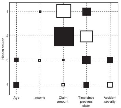
Using a Hinton diagram for variable selection involves the following steps:

1. Inspect the Hinton Diagram: Identify variables associated with weights that are close to zero, as these variables likely have minimal influence on the network’s output.
2. Iterative Removal: Remove the identified variable and reestimate the neural network. It’s often beneficial to start the reestimation process using the previous weights to speed up convergence.
3. Reevaluation: Continue to inspect the updated Hinton diagram, removing additional variables and reestimating the network until a predetermined stopping criterion is met. This criterion might be based on a significant decrease in predictive performance or after a certain number of iterations.

This process helps in refining the neural network, potentially improving its performance by eliminating variables that do not contribute significantly. For a more systematic approach to variable selection in neural networks, consider the following steps:

1. Initial Network Construction: Begin by building a neural network that includes all available variables ( variables).
2. Sequential Variable Removal: Remove each variable one by one, reestimating the network each time. This will produce networks, each containing variables.
3. Performance Evaluation: Assess the performance of each network using metrics such as misclassification error (for classification tasks) or mean squared error (for regression tasks).
4. Selection of Optimal Variable: Identify and remove the variable whose exclusion leads to the best-performing network.
5. Iteration: Repeat the process of variable removal and performance evaluation until removing additional variables results in a significant decrease in model performance.

Variable selection can be computationally expensive, especially with large datasets or complex neural networks. To mitigate this, sampling techniques can be employed to reduce resource consumption. For instance, rather than evaluating every possible variable, one might randomly sample subsets of variables or data points to estimate their impact on model performance. This approach can significantly speed up the selection process while still providing a reliable assessment of variable importance.

Rule Extraction Procedure

To gain interpretability from a neural network, extracting if-then classification rules can be highly effective. There are two primary techniques for this extraction:

1. Decompositional Technique: This method involves breaking down the neural network’s internal structure to understand how it makes decisions. It focuses on the following:

   • Weight Analysis: Examine the weights of the connections between neurons. By understanding how these weights influence the network’s output, you can infer the rules that the network follows.
   • Activation Values: Analyze the activation values of neurons in response to different inputs. This helps in identifying patterns and thresholds that contribute to decision-making.

   

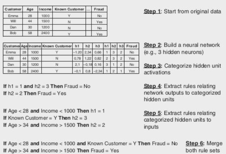
   By synthesizing this information, you can derive rules that approximate the neural network’s decision-making process. This approach requires a deep understanding of the network’s architecture and parameters.

2. Pedagogical Technique: Here, the neural network is viewed as a “black box”, meaning its internal workings are not directly analyzed. Instead:

   • Black Box Behavior: The network’s inputs and outputs are observed to determine how it makes predictions.
   • White-Box Technique: A more interpretable model, such as a decision tree, is trained using the same input-output pairs as the neural network. The decision tree then provides a set of if-then rules that approximate the network’s behavior.

   

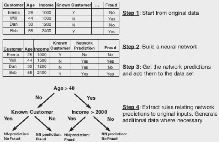
   This technique allows for the generation of easily understandable rules without needing to decipher the network’s internal parameters directly.

Once you have extracted a set of rules, their effectiveness must be assessed through several criteria:

• Accuracy: Measures how well the extracted rules predict the correct classifications compared to the neural network.
• Conciseness: Evaluates whether the rules are simple and understandable, avoiding unnecessary complexity.
• Fidelity: Assesses how closely the rules match the neural network’s decision-making. It is calculated using the formula: where: - is the number of correctly classified instances by both the rules and the network. - is the number of correctly rejected instances (i.e., instances not classified by the network but rejected by the rules). - is the number of incorrectly classified instances by the rules. - is the number of incorrectly rejected instances by the rules.

To validate the extracted rules or decision trees:

• Comparison with Directly Trained Trees: Build a decision tree directly from the original data and compare its performance to the rules derived from the neural network. This comparison helps gauge the effectiveness of the rule extraction process.

Two-stage Model Setup

To achieve an ideal balance between model interpretability and performance, a two-stage model can be implemented.

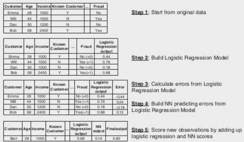
In the first stage, an easy-to-understand model such as linear regression or logistic regression is estimated. This model provides interpretability and insights into the relationship between predictors and the target variable. In the second stage, a neural network is used to predict the errors made by the simple model, using the same set of predictors. This nonlinear model captures complex patterns and improves the overall performance of the model.

The two models are then combined in an additive way, leveraging the strengths of both. This approach allows for a more interpretable understanding of the model’s behavior while benefiting from the enhanced predictive power of the neural network.

Support Vector Machines

Support vector machines (SVMs) were developed as an alternative to neural networks to address their limitations. Unlike neural networks, SVMs have a convex objective function, which means they do not suffer from the issue of multiple local minima. Additionally, SVMs do not require tuning the number of hidden neurons, making them easier to work with.

The concept of SVMs can be traced back to the field of linear programming. SVMs utilize an objective function and constraints to find an optimal decision boundary that separates different classes of data. By maximizing the margin between classes, SVMs aim to achieve better generalization and robustness in classification tasks.

SVMs can handle both linearly separable and non-linearly separable data. In the case of linearly separable data, SVMs aim to find a hyperplane that maximizes the margin between classes. For non-linearly separable data, SVMs use kernel functions to map the data into a higher-dimensional feature space, where a linear separation can be achieved.

One advantage of SVMs is their ability to perform variable selection. By analyzing the weights associated with each variable, SVMs can identify the most influential features in the classification process. This can be useful for understanding the underlying factors driving the classification decision.

Linear Programming: Key Problem

The key problem in linear programming is to estimate multiple optimal decision boundaries for a perfectly linearly separable case. Support Vector Machines (SVMs) address this problem by adding an extra objective to the analysis.

In the linear separable case, SVMs aim to maximize the margin between the decision boundaries (hyperplanes) to pull both classes as far apart as possible. The support vectors are the training points that lie on one of the hyperplanes, while the classification hyperplane is denoted as .

When new observations are encountered, they are checked to see if they are situated above , in which case the prediction is , or below , in which case the prediction is .

Linear Separable Case

In Support Vector Machines (SVMs), the linear separable case refers to a scenario where the classes of data can be perfectly separated by a linear decision boundary. The objective in this case is to find the optimal decision boundary that maximizes the margin between the classes.

The optimization problem in the linear separable case can be formulated as follows:

Here, the objective function aims to minimize the sum of squared weights, while the constraints ensure that each data point is correctly classified with a margin of at least 1.

This optimization problem is convex, meaning it has a unique global minimum and no local minima. As a result, SVMs in the linear separable case provide a reliable and robust solution for classification tasks.

The Linear Non-separable Case

In scenarios where class distributions overlap, the SVM classifier can be extended with error terms. This allows for misclassifications by introducing error variables. The objective function now includes a term that balances the importance of maximizing the margin and minimizing the error on the data. The hyperparameter controls this balance, with a higher value of implying a higher risk of overfitting.

For cases where interpretability is crucial, nonlinear SVM classifiers can be used. These classifiers map the input data to a higher dimensional feature space using a mapping function . While they offer a universal approximation property and do not require tuning the number of hidden neurons, they involve complex optimization and may lack interpretability. Variable selection in SVMs can be performed using the backward variable selection procedure. However, this procedure only reduces the variables and does not provide additional insight into the workings of the SVM.

Rule extraction approaches, such as decompositional methods, can represent SVMs as neural networks. The hidden layer of the network uses kernel activation functions, with the number of hidden neurons automatically determined by the optimization process. The output layer employs a linear activation function.

A pedagogical approach can be combined with SVMs to enhance comprehensibility. In this approach, the SVM is first used to construct a dataset with predictions for each observation. This dataset is then fed into a decision tree algorithm to build a decision tree. Additional training set observations can be generated to facilitate the tree construction process.

Two-stage models can also be employed to provide a more comprehensive understanding. In this approach, a simple model, such as linear or logistic regression, is estimated first. Then, an SVM is used to correct the errors made by the simple model. This combination leverages the strengths of both models, resulting in improved interpretability and performance.

Ensemble Methods

Definition

Ensemble methods are techniques that involve estimating multiple analytical models instead of relying on a single model. By using multiple models, ensemble methods aim to cover different parts of the data input space and complement each other’s deficiencies.

This approach is particularly effective when the underlying data is subject to changes. Ensemble methods are commonly used in conjunction with decision trees. There are several popular ensemble methods:

1. Bagging: Bagging, short for bootstrap aggregating, involves creating multiple bootstrap samples from the original dataset and building a classifier for each sample. The final prediction is made by combining the predictions of all the classifiers, either through voting (for classification problems) or averaging (for regression problems).
2. Boosting: Boosting is an iterative process that starts with equal weights assigned to each data point. In each iteration, the weights are adjusted based on the classification error, giving more weight to misclassified cases. The final ensemble model is a weighted combination of all the individual models.
3. Random Forests: Random forests create a forest of decision trees. Each tree is trained on a random subset of attributes at each node, and the final prediction is made by aggregating the predictions of all the trees. The diversity among the base classifiers in terms of training samples and attribute subsets leads to improved performance compared to using a single model.

Ensemble methods have been widely studied and evaluated in various benchmarking studies. Random forests, in particular, have shown excellent performance in many applications.

Bagging (Bootstrap aggregating)

Bagging, short for bootstrap aggregating, is an ensemble method that involves creating multiple bootstrap samples from the original dataset and building a classifier for each sample. The number of bootstraps, denoted as , can be fixed or tuned using an independent validation dataset.

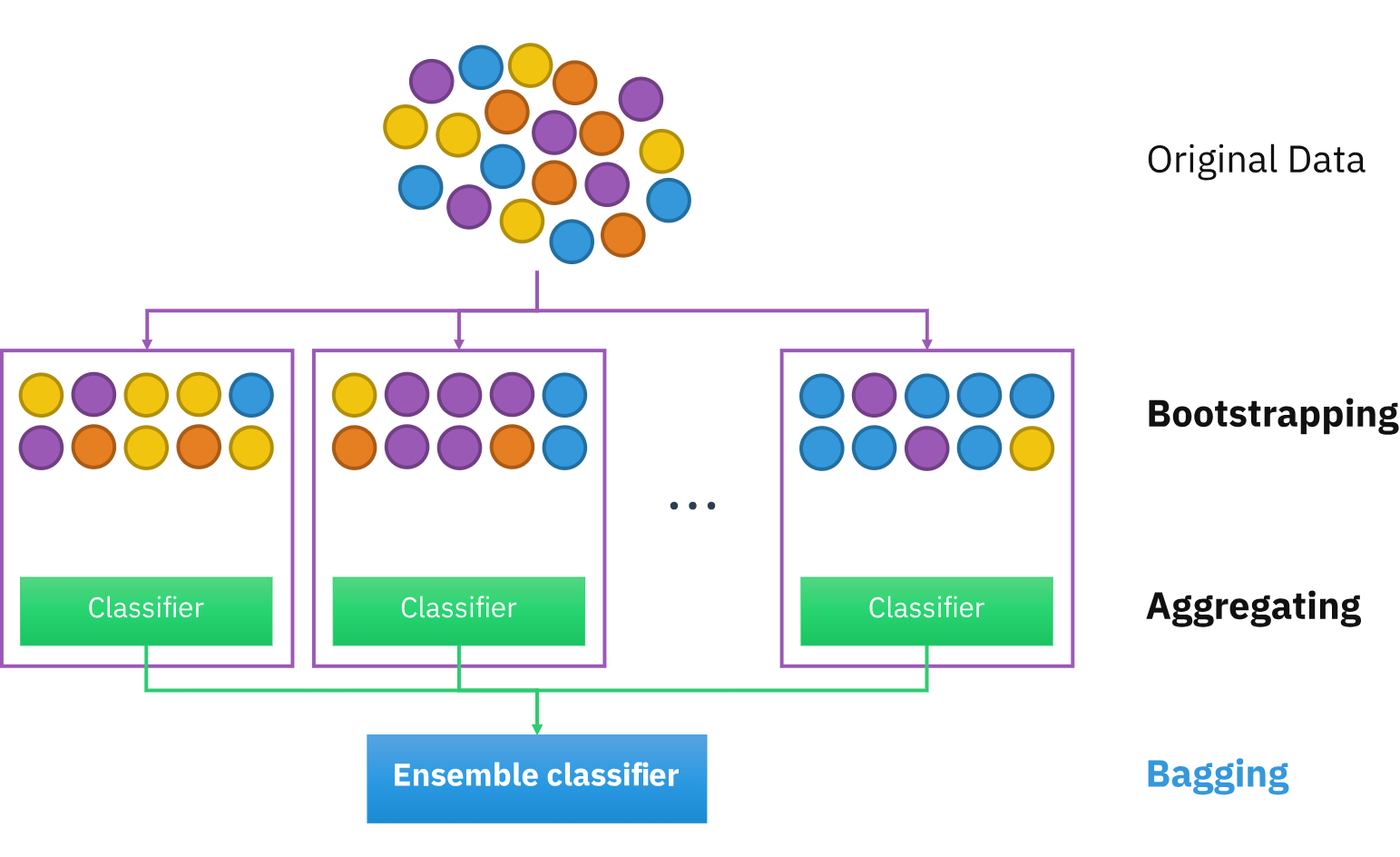
In bagging, each bootstrap sample is created by randomly selecting observations from the original dataset with replacement. This process introduces variability into the training data, which can improve the accuracy of the resulting models. For classification tasks, the final prediction is made by combining the predictions of all the classifiers through voting. In regression tasks, the prediction is the average of the outcomes predicted by the individual models.

The effectiveness of bagging depends on the instability of the underlying analytical technique. If perturbing the data set through bootstrapping can significantly alter the model constructed, bagging can provide improved accuracy. However, for models that are robust to variations in the data, bagging may not offer significant benefits.

Bagging has been widely used and studied in various domains, including fraud detection. It is particularly useful when dealing with complex datasets or when high-performing analytical methods are required. By leveraging the diversity among the base classifiers, bagging can enhance the overall predictive performance of the ensemble model.

Boosting: An Ensemble Method for Fraud Detection

Boosting is an ensemble method that involves estimating multiple models using a weighted data sample. The goal of boosting is to iteratively re-weight the data based on the classification error, giving more attention to difficult observations. This approach is particularly useful in fraud detection, where identifying challenging cases is crucial.

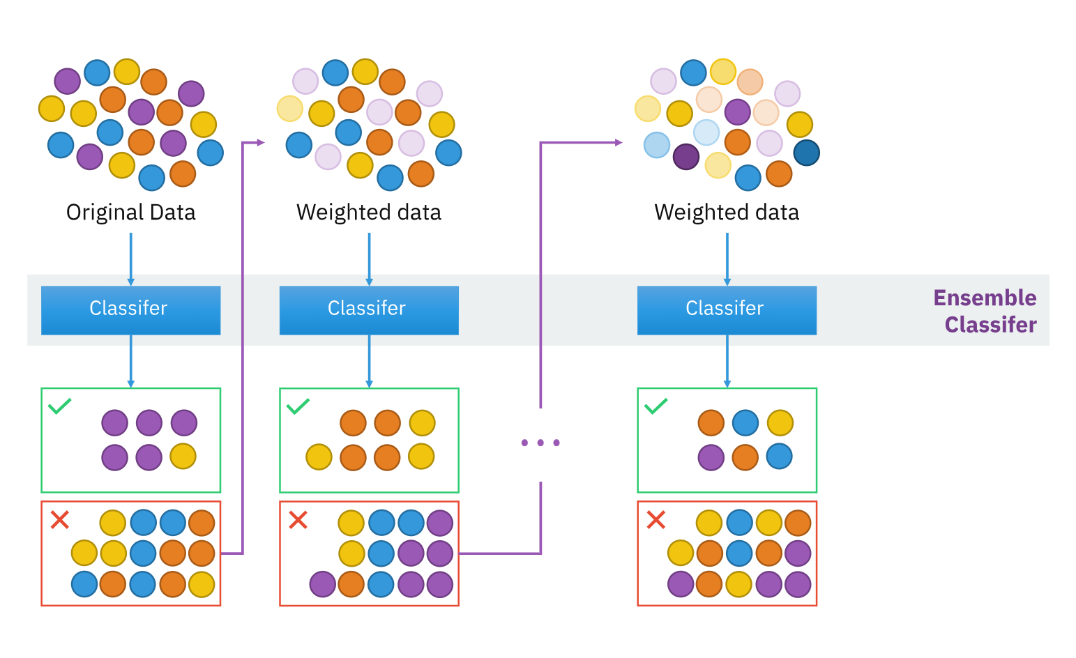
The boosting algorithm starts with uniform weights assigned to each data point. In each iteration, the weights are adjusted based on the classification error, giving higher weights to misclassified cases. The final ensemble model is a weighted combination of all the individual models.

One popular implementation of boosting is the Adaptive Boosting (Adaboost) procedure. The number of boosting runs can be fixed or tuned using an independent validation set.

While boosting is easy to implement, it has a potential drawback. There is a risk of overfitting to the hard examples in the data, which can be noisy in a fraud detection setting. Therefore, careful consideration should be given to the noise level in the target labels when applying boosting for fraud detection tasks.

Boosting is a powerful technique that can enhance the performance of fraud detection models by focusing on challenging cases and improving overall accuracy.

Random Forests

Random Forests is an ensemble learning technique that builds a collection of decision trees to improve predictive accuracy. It leverages important principles like diversity among base classifiers, random selection of attributes at each node, and the strength of individual models. The diversity among classifiers is achieved through a bootstrapping procedure that selects different training samples for each classifier, introducing variability into the training data and resulting in a range of diverse models. At each decision tree node, a random subset of attributes is chosen for splitting, which further increases the diversity among the classifiers.

The strength of individual models is another critical factor in the overall performance of the ensemble. Each model is trained on a distinct subset of data, enabling them to capture different aspects of the underlying patterns. This combination of diverse and strong base models results in an ensemble that generally outperforms individual models. The variety among classifiers allows the ensemble to cover different parts of the data input space and compensate for each other’s weaknesses. Random Forests have been extensively studied and consistently demonstrate excellent predictive performance across various domains. They are particularly recommended for high-performing analytical tasks such as fraud detection.

Random forests have consistently demonstrated excellent predictive performance in various benchmarking studies. They consistently rank among the top-performing models across a wide range of prediction tasks. Random forests excel in handling datasets with a small number of observations but a large number of variables. They are particularly recommended for fraud detection tasks that require high-performing analytical methods.

However, one drawback of random forests is their black-box nature. Due to the ensemble’s composition of multiple decision trees, it can be challenging to understand how the final classification is made. To gain insights into the internal workings of a random forest, one approach is to calculate the variable importance (VI). VI provides information on the relative contribution of each variable in the ensemble’s decision-making process, shedding light on which variables are most influential in the classification outcome.