Text Classifier

Small introduction of Machine Learning and supervised learning

Definition

Machine Learning (ML) is a technique aimed to make machines “act more intelligent” by generalizing from past data to predict future data.

A standard definition for ML is:

Quote

“A computer program is said to learn from experience with respect to some class of tasks and a performance measure , if its performance at tasks in , as measured by , improves because of experience .”

- Tom M. Mitchell

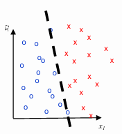
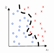
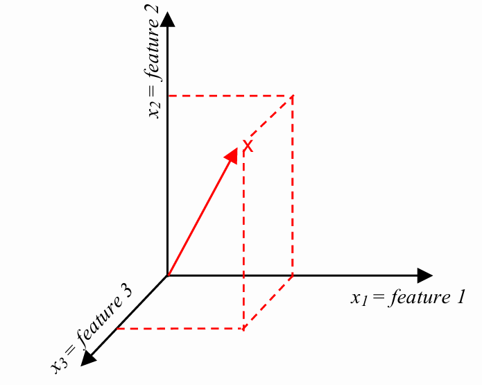
A common task for ML is classification. In this task, the goal is to partition the feature space into regions, each corresponding to a different class. In supervised learning, each training instance is a point in some feature space, and each training instance has been labeled with a class. The goal is to partition the space to make future predictions. But, in many cases, the data overlaps, so classes are not linearly separable; another cases, the instances has too many features and some dimensions are better at distinguishing classes than others.

Training a Model

To train a model, the following steps should be followed:

1. Provide the training instances and their corresponding labels to the learning algorithm. The algorithm will search for the best parameter settings of the model to minimize prediction error for the labels.
2. The outcome of the learning algorithm is a model that can be utilized to predict the labels of new instances (test).

flowchart TB
    TrainInstances[(Train<br>Instances)] --> LearningAlgorithm[Learning<br> Algorithm]
    TrainLabels[(Train<br>Labels)] --> LearningAlgorithm

    LearningAlgorithm --> Model((Model)) 
    Model --> Apply
    NewInstances[(New<br>Instances)] --> Apply

    Apply --> Predictions

The classification of models can be divided into two categories:

1. Linear Models: These models are represented as a linear combination of the input features. They create a hyperplane that partitions the feature space into different regions, each associated with a specific class. Examples of linear models include Naive Bayes, Logistic Regression, and Support Vector Machines.

   

2. Non-linear Models: These models are represented as a non-linear combination of the input features. They create a surface that partitions the feature space into different regions, each associated with a specific class. Examples of non-linear models include Gradient Boosted Decision Trees and Neural Networks.

   

In machine learning, overfitting is a critical problem that arises when a model becomes excessively complex. This complexity often leads to the model performing exceptionally well on the training data, as it captures not just the underlying patterns but also the noise and specific details of the training set. While this might initially seem advantageous due to the reduced training error, it becomes detrimental when the model is applied to unseen data. As a result, the test error — which measures the model’s performance on new, unseen data — begins to increase. This increase indicates that the model is not generalizing well, meaning it has learned to perform well only on the training data, not on new data.

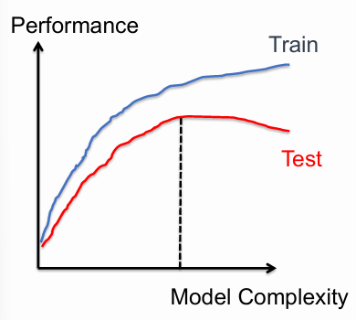
Conversely, underfitting occurs when a model is too simplistic to accurately capture the underlying patterns in the data. A model that is underfitting will have both high training and test errors because it fails to represent the complexities inherent in the data. This usually happens when the model’s capacity is too low, such as when using a linear model to fit a non-linear relationship

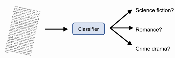
Text Classification

Definition

Text classification is the process of training a model to predict the class of a text.

This is a really common task in NLP, and it’s used for:

• spam detection (applied to emails)
• authorship attribution (applied to books)
• sentiment analysis (applied to reviews)
• offensive content detection (applied to social media)
• web search query intent classification (applied to search queries)
• personalized news feed (applied to news articles)
• identifying criminal behavior (applied to chat logs)
• routing communication to the right department (applied to customer support)

Types of text classification problems:

• Binary classification: The text is assigned to one of two classes. This is the simplest case of text classification and it’s used in spam detection, sentiment analysis, etc.
• Multi-class classification: The text is assigned to one of many classes. This is used in authorship attribution, web search query intent classification, etc.
• Multi-label classification: The text is assigned to one or more classes. This is used in offensive content detection, personalized news feed, etc.
• Ordinal classification: The text is assigned to one of many ordered classes. This is used in rating prediction, etc.

Extracting Features from Text

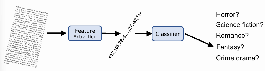
Given an arbitrary long text, it cannot be given directly to a model. The text must be converted into a fixed-length vector of numbers, by passing through a feature extraction process; then, a classifier can be trained on these vectors in order to find the features that best predict the class of the text.

Definition

Features are signals in documents that are useful for predicting category.

We need to convert text data into a vector of features to give to the classifier. If training data is scarce (few documents available) one might use:

• Syntax based features (eg. number of words, number of sentences, number of paragraphs)
• Part of speech features (eg. number of nouns, number of verbs, number of adjectives)
• Reading difficulty based features (eg. Flesch-Kincaid readability score, Gunning Fog index)

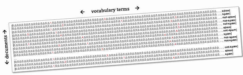
Most common feature to extract are words themself. The vocabulary of document provides important signals and the number of occurrences of words provides further information. The simplest way to convert text into a vector of features is to use the bag of words model. This model represents a document as a vector of word counts, where each element of the vector corresponds to the number of times a word appears in the document.

The bag of words model is simple and effective, but it has some limitations: it does not take into account the order of words, the meaning of words, and the context of words.

Preprocessing Text for classification

The preprocessing phase is common, but not necessary for all text classification tasks. It is used to clean the text and to make it more suitable for the feature extraction phase. The preprocessing phase usually consists of the following steps:

• before the tokenization, we need to remove all the mark-up and non-textual content from the text, lowercasing the text, and removing all the punctuation.(“;.&%$@!<>?...”)
• after the tokenization, we need to remove all the stopwords, low frequency words, perform some sort of stemming/lemming and fix all the spelling errors.

Bag of Words representation

Documents are sequences of categorical variables (words of vocabulary). Usually, in ML we one-hot encode the categorical variables, providing new binary feature for every possible value of categorical variable. In the case of large text however, to one-hot encode a sequence of categorical variables with a vocabulary of thousand would require million columns; so there are too many features given small amount of training data vailable. So, to reduce the space complexity, we have to sum all the one-hot encodings together: that reduces the number of columns to the size of the vocabulary and throws away all word order information but retains critical vocabulary information.

The vocabulary of a document is very small compared to the vocabulary of the collection, so the terms present in document usually characterize well content of the document. BOW representation include also the count of occurrences of each term in the document, so the BOW representation is a vector of the size of the vocabulary, where each element of the vector corresponds to the number of times a word appears in the document. This could use binary representation of document with little information loss.

BOW completely ignores the order of words in the document. Extension to include an -gram (bigram, trigram, etc.) representation of the document can increase the performance of the classifier, but greatly increase the number of dimensions of the feature space, so more data is the needed to train the model.

Usually, have far fewer documents than vocabulary terms, which means that we have fewer examples the features, so the model is more likely to overfit. To prevent overfitting, we can use the held-out validation portion of the training set to prevent overfitting by finding hyperparameters value that maximize the generalization performance.

Linear classification models

Definition

A linear classifier is a classifier that makes its predictions based on a linear combination of the input features.

Linear models are often used with text because of the very high number of dimensions in the bag-of-words representation. They are simple and interpretable, and they can be trained quickly on large datasets. They are also robust to overfitting, can be regularized to prevent overfitting, and can be used to extract feature importance.

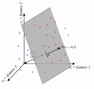
Linear classification algorithms are designed to identify linear decision boundaries. In other words, these models create a hyperplane in an -dimensional vector space that partitions the feature space into distinct regions, each associated with a specific class.

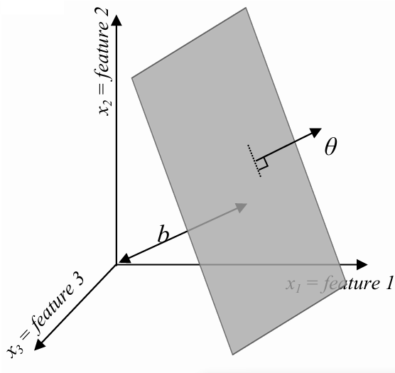
Given a feature vector and a set of model parameters , the oriented hyperplane is defined by the equation , where

• is the dot product between the feature vector and the model parameters
• is an -dimensional vector that is orthogonal to the hyperplane
• is the offset term, indicating the distance of the hyperplane from the origin. If , then is the distance of the hyperplane from the origin, otherwise the distance is . is just another parameter of the model and usually is denotated as .

Multinomial Naive Bayes (NB)

Naive Bayes (NB) is one of the oldest and simplest text classifiers. It is based on Bayes’ theorem, which describes the probability of an event, based on prior knowledge of conditions that might be related to the event. The NB classifier is called “naive” because it makes the simplifying assumption that

word courrences are statically independent of each other, given the class label.

This means that words provide independent information about the class label, and that the presence of a word in a document does not affect the presence of other words in the document.

However, this assumption is not true in practice, since the words are highly correlated with each other, but nonetheless the prediction from the model are good.

The multinominal NB want to estimate the probability of spam given the text content of the email: . This probability can’t estimate the class probability directly, because haven’t seen any email exactly like it before (with the same set of words). So, use the Bayes rule to swap the order of the events:

We can ignore the denominator, because it’s the same for both spam and not spam, and we can normalize later

Now, we make simply (and clearly wrong) assumption that words occurences are not correlated within the classes, it means that we assume that , so we can write

Finally, we can estimate the probability from the training data, by counting the number of times each word appears in the spam and not spam emails, and then normalizing the counts to get the probabilities.

If all examples of a word occur for only one class, then the probability of the word given the other class is zero, so the probability of the document given the other class is zero, and doesn’t make sense since we may just have not seen enough examples of the other class. To prevent this, we can use Laplace smoothing, which adds a small constant to the counts of each word in the training set, so that the probability of a word given a class is never zero. can be chosen to maximize prediction performance or set to default value. If , then the probability of a word given a class is the same as the probability of a word given the other class, so the model is not biased towards any class.

If a new word appears in test set, but not in the training set, then the probability of the word given the class is zero, so the probability of the document given the class is zero, and the model can’t make a prediction. To prevent this, we can use add-one smoothing, which adds one to the counts of each word in the training set, so that the probability of a word given a class is never zero.

How is NB a linear classifier?

Naive Bayes computes product of conditional probabilities of words in document:

Considering both classes together, we can calculate the odds of spam as:

Taking the will convert the product into a sum, and summing over the vocabulary (features) rather than position within the document it giving us a linear equation of the document feature vector :

This is the standard linear equation for a linear classifier: and classify as spam if .

Let’s talk about for one moment about the independence assumption. The spamming classifier as presented before uses the presence of words as feature. The independence assumption posits that knowing whether spam email contains a particular word, as “cheap”, doesn’t change the probability of seeing words like “save”: . This is clearly not true, because the words are correlated with each other, but simplifies problem of estimating model and making predictions. The presence of “cheap” in the email, can increase the spam score by and the presence of “save” only by ; seeing both “cheap” and “save” increase the spam score by , so the model can still make good predictions.

Pros and Cons of Naive Bayes

Pros:

• very fast to estimate NB model, because it requires only one pass over the training data and no need to search for parameters
• reliable predictor even if there is little data available (if conditional independence assumption holds, it’s the best)

Cons:

• doesn’t tend to perform quite as well on large data as other classifiers, especially if many redundant features since information is being counted twice
• predicted probabilities are not well calibrated, they tend to be too overconfident due to violations of indipendence assumption

Logistic Regression

In machine learning, when making predictions, the certainty of a prediction increases as the distance of a data point from the decision boundary grows. The decision boundary is the surface that separates different classes — in this case, fraud and non-fraud. The further a point is from this boundary, the more confident the model is about the classification.

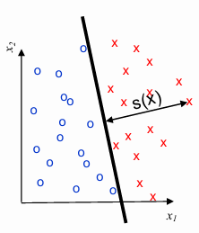
The signed distance of a point from the decision boundary (or hyperplane) can be mathematically expressed as:

where represents the weight vector that defines the orientation of the hyperplane, is the bias term that shifts the hyperplane and is the input feature vector.

The sign and magnitude of provide insight into the classification:

• A positive value of suggests that the point is likely classified as fraud.
• A negative value of indicates that the point is likely classified as non-fraud.
• The magnitude of reflects the confidence in the prediction—the larger the magnitude, the more confident the model is.

Instead of merely classifying a point as fraud or non-fraud, it is often useful to estimate the probability that a given point is fraudulent. This probability can be interpreted as the model’s confidence in its classification. To do this, we need to convert the signed distance into a probability value , which ranges between and . This conversion requires a function that can map the entire real number line to the interval . The logistic function (also known as the sigmoid function) is ideal for this purpose because it has the necessary properties: where is the signed distance . The function’s output is always between and , making it perfect for probability estimation.

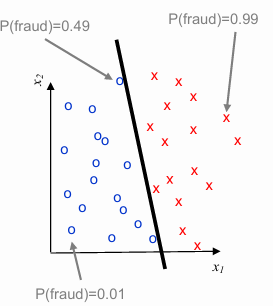
At the decision boundary, where the signed distance is equal to 0, the sigmoid function outputs a probability of . This means that the model is equally uncertain about whether the point belongs to the fraud or non-fraud class. The slope of the sigmoid function, which determines how quickly the probability changes as the signed distance changes, is influenced by the magnitude of the weights . A larger value of results in a steeper curve, leading to sharper transitions between probabilities near the decision boundary.

Definition

The Logistic regression (LR) is a very popular algorithm for learning a statical classifier. It requires a set of numerical features and assumes that the log-odds of class label is a linear function of feature values.

LR uses linear model (distance from hyperplane) to predict the log-odds:

If we invert the log-odds function, we get the logistic function:

Log-odds to predicted probability is a linear function . When the probability is , log-odds is , classifies point as positive if log-odds is positive, so LR learn a linear decision boundary. Changing the value of a feature, increase or decrease predicted probability monotonically depending on whether coefficient is positive or negative.

Pros and Cons of Logistic Regression

Pros:

• produces well-calibrated probability estimates
• can be trained efficiently and scales well to large numbers of features
• explainable since each feature’s contribution to final score is additive

Cons:

• assumes feature value are linearly related to log-odds; if assumprion is strongly violated, model will perform poorly

Support Vector Machines

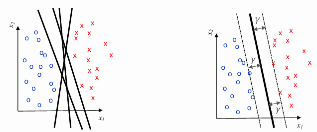
Imagine data for 2 classes split nicely into 2 groups: lots of options for where to place linear decision boundary and choose to approximately average over them should be robust and generalize well to new data. SVM finds the maximum margin hyperplane separating classes. The points lying exactly on the margin referred to as support vectors, prevent the margin from getting bigger, thus constrain/define location of boundary. In -dimensional space, we have at least support vectors.

The difference between LR and SVR is that, the position of the hyperplane depends only on closest points (convex hull of data points), and adding or moving internal points won’t effect the boundary.

Support Vector Machine is also a linear classifier, because it finds hyperplanes in feature space that best separates the two classes. But LR and NB also found linear decision: the difference is that LR use negative log-likelihood, penalizing the points proportionally to probability of incorrect prediction (including those for which prediction was correct); SVM use hinge loss, which only penalizes points that are on the wrong side (or very close to) the hyperplane.

We can compute the distance to points from the hyperplane using . For points that lie exactly on the margin we have . Assuming for simplicity that the hyperplane passes through the origin (), then the points on the margin have , where is the normal vector to the hyperplane and is the feature vector of the point. More generally we have:

• for all the positive data points
• for all the negative data points
• for all the examples where class label is

So, just need to find parameters that maximize the margin subject to the constraint . But increasing the length of the vector increases the value of , so either fix length of vector (eg ) and maximize or set and minimize subject to the constraint . Same as minimizing loss where the distance of point on wrong side of margin .is the “error” prof the prediction.

In the case of data that are not linearly separable, we simply penalize points on wrong side of the margin based on the distance from it. In support vector, points on the wrong side of the margin provide a non-zero contribution to loss function. The objective function to minimize remains almost unchanged:

where is a hyperparameter that controls the trade-off between the margin size and the number of points on the wrong side of the margin. If is large, then the model will try to classify all the points correctly, even if it means making the margin smaller. If is small, then the model will try to make the margin as large as possible, even if it means misclassifying some points.

Hinge Loss

Reordering objective (and dividing by ) gives more natural form:

• error over training data plus regularisation term that penalizes complicated models
• error function is hinge loss, applies no cost to most correctly classified points, but linearly increases with the distance from margin

Evaluating text classifiers

To evaluate the performance of a text classifier, we need to split the test set into a test instances and test labels, and then we can use the test instances to make predictions and compare them to the test labels.

flowchart TB
    TrainInstances[(Train Instances)] --> LearningAlgorithm[Learning Algorithm]
    TrainLabels[(Train Labels)] --> LearningAlgorithm

    LearningAlgorithm --> Model((Model)) 
    Model --> Apply
    NewInstances[(Test Instances)] --> Apply

    Apply --> Predictions

    TestLabels[(Test Labels)] <-- Compare --> Predictions

Given (true positive), (true negative), (false positive), and (false negative), we can compute the following metrics for evaluating text classifiers:

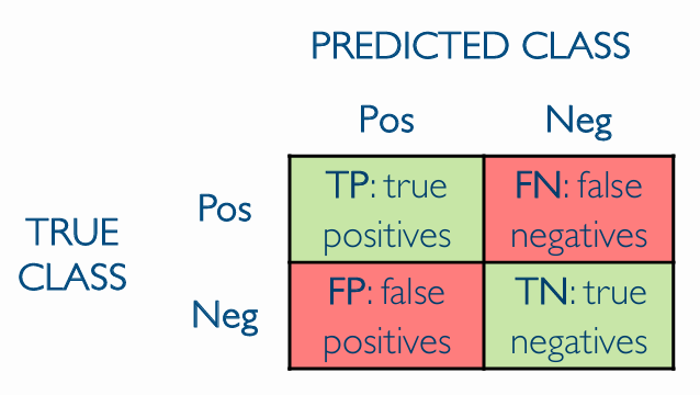
• Accuracy: the percentage of correct predictions as
• Precision: the percentage of positive predictions that are correct as
• Recall: the percentage of positive instances that are correctly predicted as
• F-measure: the harmonic mean of precision and recall as
• AuC: the area under the ROC curve, which is the curve that plots the true positive rate against the false positive rate as the threshold for classifying a point as positive is varied

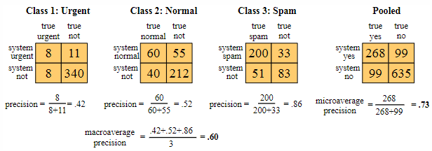
If there are three classes, the confusion matrix will have dimensions of . To calculate precision and recall values for each class, we can consider each class as the positive class in a one-versus-rest setting.

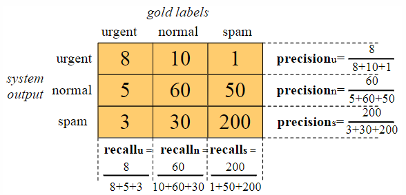
Combine precision and recall from three classes to obtain a single metric. There are two approaches to do this:

1. Macroaveraging: Calculate the performance (precision and recall) for each class individually, and then take the average across all classes.
2. Microaveraging: Combine the decisions for all classes into a single confusion matrix. From this matrix, compute the overall precision and recall.