When it comes to evaluating predictive models, there are two important decisions that need to be made.
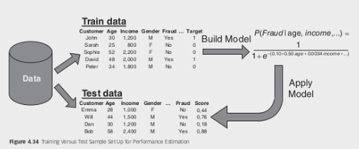
The first decision involves determining how to split up the data set. This decision depends on the size of the data set. For large data sets, it is common to split the data into a training dataset (70%) to build the model and a test dataset (30%) to calculate its performance. In cases where strict separation is required, a validation sample can also be used during model development. For small data sets, special schemes like cross-validation or leave-one-out cross-validation may be adopted.
The second decision revolves around selecting the appropriate performance metrics. There are several metrics that can be used to evaluate the performance of a predictive model. These include classification accuracy, classification error, sensitivity, specificity, and precision. Additionally, the Receiver Operating Characteristic (ROC) curve and the Area Under the Curve (AUC) provide a comprehensive measure of performance. Other factors to consider when evaluating models include interpretability, justifiability, and operational efficiency.
Splitting Up the Data Set
When preparing data for performance evaluation of a machine learning model, the method of splitting the data depends largely on the size of the dataset. Here’s a more detailed overview of common strategies for splitting data:
- For large datasets, a common approach is to divide the data into a training set and a test set. Typically,
of the data is allocated to the training set, which is used to build and train the machine learning model by identifying patterns and relationships within the data. The remaining of the data is reserved for the test set, which is used to evaluate the performance of the trained model by comparing its predictions against this held-out data. The test set provides an estimate of how well the model will perform on unseen data. In scenarios where model fine-tuning or hyperparameter optimization is required, a separate validation set can be used. This set is distinct from both the training and test sets and aids in making decisions such as when to stop training in algorithms like decision trees or neural networks. The validation set helps in tuning the model to achieve better performance without overfitting. - For smaller datasets, cross-validation methods are often preferred to maximize the utility of the available data. One common method is K-fold cross-validation, where the dataset is divided into
equal-sized folds (commonly or ). The model is trained on folds and validated on the remaining fold. This process is repeated times, with each fold serving as the validation set once. The performance metrics from each fold are averaged to provide a comprehensive evaluation of the model’s performance. This approach helps in making efficient use of all data points for both training and validation. Another method, leave-one-out cross-validation (LOOCV), is a special case of -fold cross-validation where equals the number of data points. For each iteration, one observation is left out as the validation set, and the model is trained on the remaining observations. This results in models being trained and validated. LOOCV provides a thorough performance assessment but can be computationally intensive for large datasets.
Particularly important for imbalanced datasets, such as those encountered in fraud detection, is the use of stratified cross-validation. This approach ensures that each fold maintains the same proportion of classes (fraud vs. non-fraud) as the original dataset. By maintaining the distribution of classes across folds, stratified cross-validation helps in providing a more reliable estimate of model performance.
Model Selection
When applying cross-validation to develop and evaluate multiple models, a critical decision arises: which model should be chosen as the final model for deployment or further analysis? Here are several approaches to address this:
- Ensemble Approach: One method is to use all the models generated during cross-validation in an ensemble setup. In this scenario, each model contributes to the final prediction through a weighted voting mechanism. This approach capitalizes on the collective strength of individual models, potentially improving overall performance and robustness. For instance, in a weighted voting system, models that perform better on cross-validation might have a higher influence on the final prediction.
- Leave-One-Out Cross-Validation: Another technique involves performing leave-one-out cross-validation (LOOCV) where each model is trained on all but one observation. In this setting, the final model can be selected randomly from those generated, given that they are highly similar due to only one observation difference. Since the models are almost identical, this randomness does not substantially affect the performance outcome.
- Final Model Construction: An alternative strategy is to train a single final model using the entire dataset. Although this model utilizes all available data, it is crucial to evaluate its performance using the cross-validation results. Cross-validation provides an independent estimate of performance by testing the model on unseen data subsets, which ensures that the reported performance metrics reflect how well the model generalizes to new data.
Performance Metrics
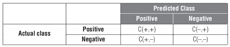
In the context of fraud detection, it is important to evaluate the performance of a predictive model using various metrics. One common approach is to use a default cut-off value of
The confusion matrix provides a comprehensive overview of the model’s performance. It consists of four elements: true positives (
- Classification accuracy: The percentage of correctly classified observations, given by
. - Classification error: The complement of accuracy, also known as the misclassification rate, given by
. - Sensitivity: Also known as recall or hit rate, it measures how many of the actual fraudsters are correctly labeled as fraudsters, given by
. - Specificity: It measures how many of the non-fraudsters are correctly labeled as non-fraudsters by the model, given by
. - Precision: It indicates how many of the predicted fraudsters are actually fraudsters, given by
.
Example
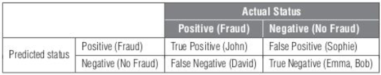
It is important to note that these classification measures depend on the chosen cut-off value. To illustrate this, consider a fraud detection example with a five-customer data set. When using a cut-off of
To overcome the dependence on the cut-off, it is desirable to have a performance measure that is independent of this threshold. This allows for a more robust evaluation of the model’s performance.
Receiver Operating Characteristic (ROC) Curve
The ROC curve is a graphical representation of the sensitivity (true positive rate) versus
When plotting the ROC curve, a problem arises if the curves intersect, indicating that the model’s performance is not consistent across different thresholds.
The Area Under the Curve (AUC) is a commonly used metric to quantify the performance of the ROC curve. It provides a simple figure-of-merit for the model’s discrimination ability. The AUC ranges from
A good classifier should have an ROC curve above the diagonal line (representing random guessing) and an AUC greater than
Other Performance Metrics
When evaluating predictive models, there are additional metrics to consider beyond classification accuracy, sensitivity, specificity, and precision. These metrics assess different aspects of the model’s performance.
- Interpretability: This metric measures how easily the model’s predictions can be understood and explained. White-box models, such as linear regression and decision trees, provide transparent and interpretable results. On the other hand, black-box models like neural networks, support vector machines (SVMs), and ensemble methods may offer higher accuracy but are less interpretable.
- Justifiability: Justifiability evaluates the extent to which the relationships modeled by the model align with expectations. It involves verifying the impact of individual variables on the model’s output. By examining the univariate impact of each variable, one can assess the justifiability of the model’s predictions.
- Operational Efficiency: Operational efficiency refers to the ease of implementing, using, and monitoring the final model. Models that are easy to implement and evaluate, such as linear and rule-based models, are preferred for fraud detection. They allow for quick evaluation and monitoring of the fraud model’s performance.
Considering these additional performance metrics alongside traditional measures can provide a more comprehensive evaluation of the predictive model’s effectiveness in fraud detection.
Developing predictive models for skewed data sets
Data sets used for fraud detection often exhibit a highly skewed target class distribution, with fraud instances accounting for less than 1% of the total observations. This poses challenges for analytical techniques, as they can be overwhelmed by the abundance of non-fraudulent observations and tend to classify every observation as non-fraudulent. To address this issue, it is recommended to increase the number of fraudulent observations or their weight, allowing the analytical techniques to give them more attention.
One approach to increase the number of fraud instances is by extending the time horizon for prediction. Instead of predicting fraud with a six-month forward-looking time horizon, a 12-month time horizon can be considered. Another method is to sample each fraud instance multiple times. For example, when predicting fraud with a one-year forward-looking time horizon, information from a one-year backward-looking time horizon can be used. By shifting the observation point earlier or later, the same fraudulent observation can be sampled twice.
The variables collected may be similar but not identical, as they are measured on a different time frame.
Determining the optimal number of fraud instances to sample is typically done through a trial-and-error process, taking into account the skewness of the target class distribution.
Under- and Oversampling
To address the issue of skewed distribution in fraud detection datasets, one approach is to replicate fraud instances two or more times. This technique, known as oversampling, increases the representation of fraud cases in the dataset, making the distribution less skewed.

Another approach to mitigate the skewness in fraud detection datasets is undersampling. In this technique, non-fraudulent instances are removed two or more times, reducing their representation in the dataset.
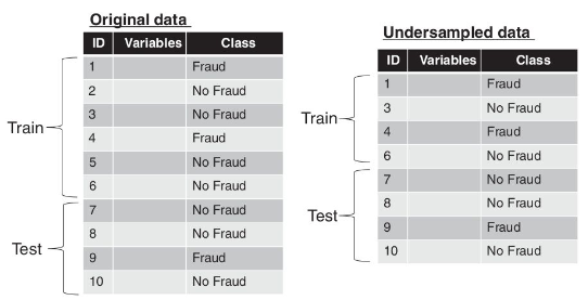
Business experience suggests removing obviously legitimate observations, such as low-value transactions or inactive accounts, to improve the performance of the model.
Under- and oversampling can also be combined to achieve a more balanced dataset. However, it is important to note that undersampling usually results in better classifiers compared to oversampling.
Determining the optimal nonfraud/fraud odds to aim for by using under- or oversampling depends on the specific dataset and the desired balance between fraud and non-fraud instances. While working towards a balanced sample with an equal number of fraudsters and non-fraudsters may seem ideal, it can introduce bias and potentially impact the model’s performance. It is generally recommended to stay as close as possible to the original class distribution to avoid unnecessary bias.
Practical Approach for Optimizing Class Distribution in Analytical Models
Determining the optimal class distribution is crucial when building an analytical model, particularly in scenarios with imbalanced data sets.
- Initial Data Assessment: Begin with your original dataset, which may exhibit a skewed class distribution. For example, in a fraud detection scenario, you might have a dataset where 95% of instances are non-fraudulent and 5% are fraudulent.
- Model Development and Evaluation: Construct an analytical model using the original dataset. Evaluate the model’s performance using the Area Under the Curve (AUC) metric, which is a common measure of a model’s ability to distinguish between classes. For a more reliable assessment, use an independent validation dataset, ensuring that the performance metrics are not overly optimistic due to overfitting.
- Class Distribution Adjustment: Alter the class distribution of your dataset by applying techniques such as oversampling the minority class (fraudulent instances) or undersampling the majority class (non-fraudulent instances). For example, you might adjust the ratio to 90% non-fraudulent and 10% fraudulent.
- Rebuild and Re-evaluate: With the adjusted dataset, develop a new model and calculate the AUC. This allows you to assess how changes in class distribution impact model performance.
- Iterative Adjustment: Continue this process of modifying the class distribution incrementally (e.g., 85% non-fraudulent / 15% fraudulent, 80% / 20%, and 75% / 25%). After each adjustment, build and evaluate a new model to record the AUC.
- Identify Optimal Distribution: Keep track of the AUC values for each class distribution adjustment. You are looking for a point where further changes in class distribution result in no significant improvement in AUC or where the AUC starts to decline. This indicates that you have likely found the optimal class distribution for your model.
Synthetic Minority Oversampling Technique (SMOTE)
Instead of simply replicating the minority observations, SMOTE takes a different approach by creating synthetic observations based on the existing minority observations. It does this by calculating the
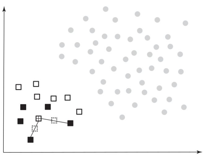
To generate the synthetic examples, SMOTE randomly creates two synthetic observations along the line connecting the observation under investigation with the two randomly selected nearest neighbors. By combining the synthetic oversampling of the minority class with under-sampling of the majority class, SMOTE aims to achieve a more balanced dataset.
Compared to traditional under- or oversampling techniques, SMOTE has been found to generally perform better in improving the performance of classifiers on imbalanced datasets.
Cost-sensitive Learning
In cost-sensitive learning, higher misclassification costs are assigned to the minority class. The idea behind this approach is to prioritize the correct classification of the minority class instances, as misclassifying them can have more severe consequences.
Typically, the misclassification costs are set such that
During the learning process of the classifier, the goal is to minimize the overall misclassification cost. By assigning higher costs to misclassifications of the minority class, the classifier is encouraged to prioritize the correct classification of minority class instances.
Cost-sensitive learning is particularly useful in scenarios where the consequences of misclassifying the minority class are more significant and need to be minimized.