9 - Attention Mechanism and Transformers

Sequence-to-sequence (Seq2Seq) models, widely used in tasks such as machine translation, text summarization, and speech recognition, often rely on a fixed source representation. However, this fixed representation can become a bottleneck, leading to suboptimal performance in both the encoder and decoder components of the model. The encoder may struggle to compress the full semantic and syntactic information of a sentence into a single, fixed representation, while the decoder may find it challenging to access the specific information needed for generating outputs at various steps. This mismatch can degrade the quality of the generated sequences, particularly for long or complex inputs.

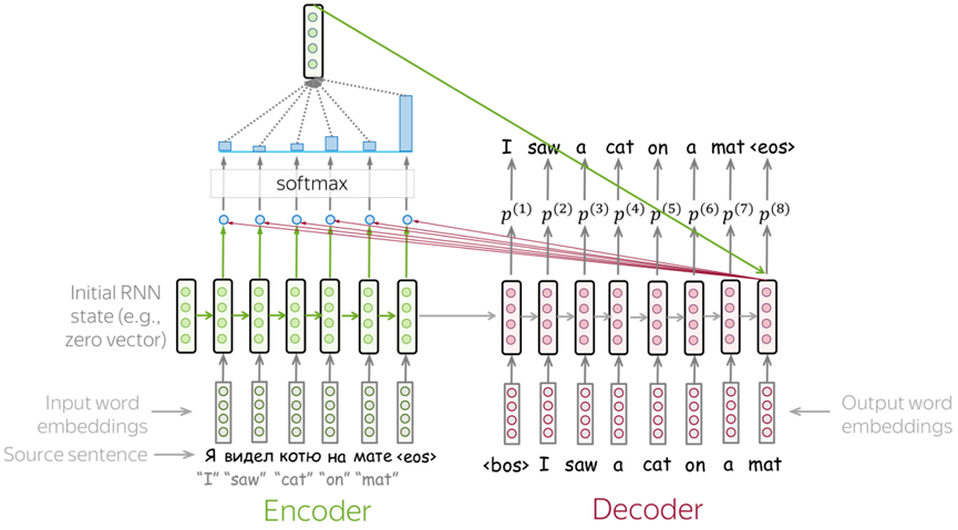
Attention mechanisms were introduced to address this limitation by allowing the model to dynamically focus on different parts of the input sequence during decoding. Instead of relying on a single static representation, the decoder uses the attention mechanism to decide which portions of the source sequence are most relevant at each decoding step. This dynamic approach enhances the model’s flexibility and improves its ability to handle complex input-output mappings.

Components of the Attention Mechanism

The attention mechanism operates through a series of well-defined computational steps:

1. Attention Input:
   The attention mechanism takes as input the set of encoder states, denoted as , where is the length of the source sequence, along with the current decoder state , which represents the decoder’s context at step . Together, these inputs enable the computation of attention scores that quantify the relevance of each encoder state to the current decoding step.

2. Attention Scores:
   Attention scores are computed to measure the relevance of a source token (from the encoder) for generating the target token at step in the decoder. These scores are computed using a scoring function, such as:

   Various scoring mechanisms have been proposed, each with distinct characteristics and computational properties.

3. Attention Weights:
   The attention scores are normalized into probabilities using the softmax function, resulting in attention weights. These weights determine the relative importance of each source token for the current decoding step :

4. Attention Output:
   Using the computed attention weights, the model generates a context vector that serves as the input for the decoder at step . This context vector is a weighted sum of the encoder states:

   The context vector effectively summarizes the relevant information from the source sequence, dynamically adapting to the needs of the decoder.

Scoring Mechanisms in Attention

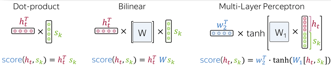
Different mechanisms for computing attention scores have been developed, each offering unique advantages and trade-offs. These include:

1. Dot-Product Attention:
   A simple and computationally efficient method, dot-product attention calculates the score as the dot product between the decoder state and the encoder state . While effective in many scenarios, it may struggle when the dimensions of and are large.

2. Bilinear Attention (Luong Attention):
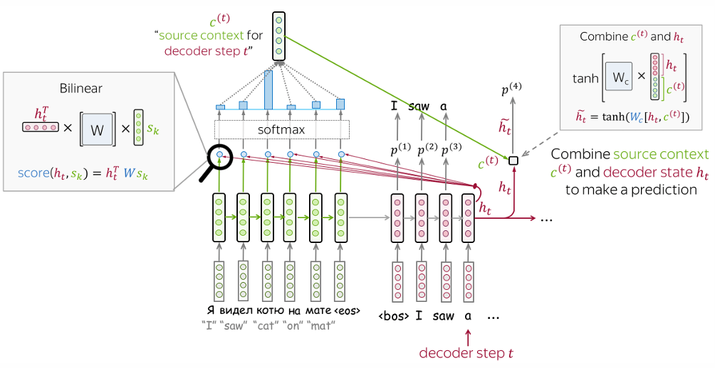
   Proposed as part of the original Luong model, bilinear attention introduces a learnable weight matrix that modulates the interaction between and :

   This approach adds flexibility by allowing the model to learn task-specific relationships between the source and target sequences.

   

3. Multi-Layer Perceptron (MLP) Attention (Bahdanau Attention):
   Introduced in the Bahdanau model, this method uses a small neural network to compute attention scores:

   This approach is more expressive and can model complex interactions, though it comes at a higher computational cost.

   

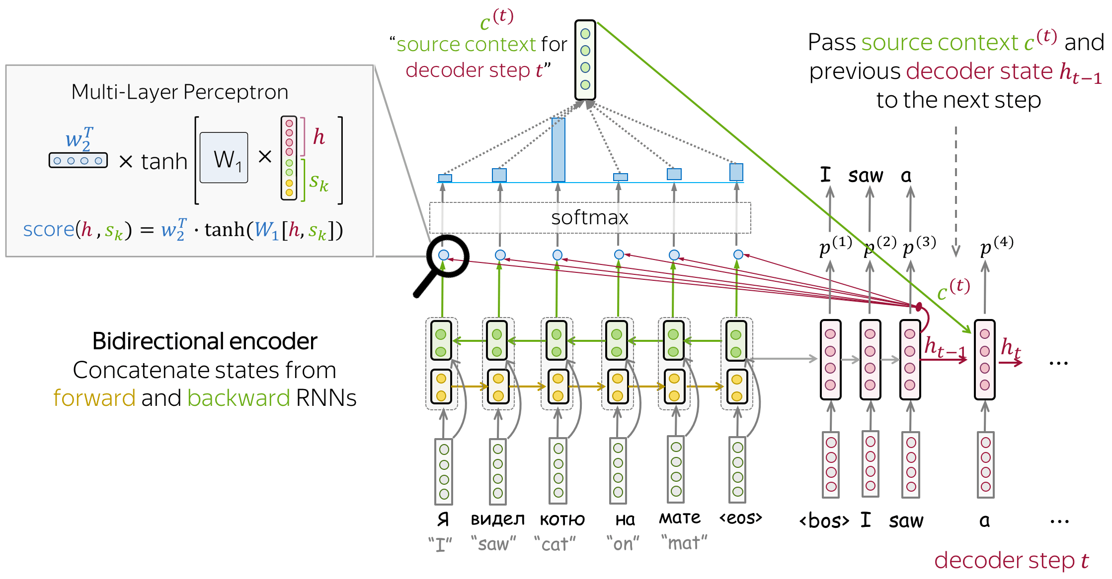
All of these methods are fully differentiable, enabling the attention mechanism to be trained end-to-end with the rest of the Seq2Seq model.

The Benefits of Attention

The attention mechanism provides a soft alignment between the source and target sequences, making it particularly effective for tasks where the correspondence between input and output is not strictly sequential. For example, in machine translation, certain words in the target language may correspond to non-adjacent words in the source language. By learning to focus on different parts of the input dynamically, attention enables the model to handle such complexities with greater accuracy.

Moreover, attention mechanisms are crucial for long sequences, where the fixed-length bottleneck of traditional Seq2Seq models becomes especially pronounced. By allowing the decoder to access the entire sequence of encoder states, attention mitigates the information loss that can occur when compressing long inputs into a single vector.

Generative Chatbots and Sequence-to-Sequence Models

Generative chatbots aim to produce human-like responses in conversations by leveraging sequence-to-sequence (Seq2Seq) models. These models can map input sequences, such as an utterance by one speaker, to output sequences, such as a reply from another speaker. For instance, if the first speaker says “ABC,” the chatbot responds with “WXYZ.”

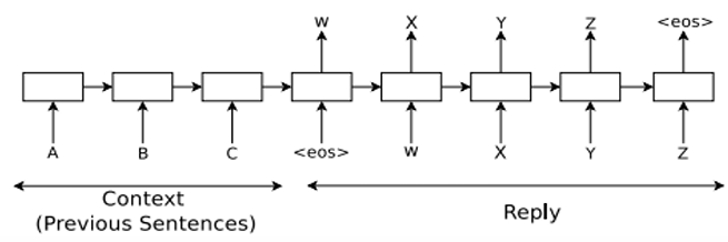
The foundational concept of generative chatbots originates from machine translation models, where a sequence in one language is translated into another. In this case, the chatbot uses an encoder-decoder architecture to encode the user’s input into a context vector and then decode it to generate the response word by word. This approach offers simplicity and generality, making it applicable to a variety of conversational tasks. Additionally, attention mechanisms are often employed to enhance the model’s ability to focus on specific parts of the input sequence, improving the relevance and coherence of responses.

Response Generation and Context Handling

Chatbots can be categorized based on two key dimensions: response generation and context handling.

Response Generation Strategies

Chatbots typically generate responses using one of two core algorithms: generative models or retrieval-based models:

• Generative Models:
  Generative chatbots create responses from scratch by modeling the probability distribution of the output sequence, conditioned on the input sequence. These models encode the input question into a context vector and generate the answer word by word. For example, an encoder-decoder model with an attention mechanism generates responses by predicting the most probable next word in the sequence at each step. This approach allows for more flexible and creative responses but requires extensive training data to ensure grammatical and contextually appropriate output.

• Retrieval-Based Models:
  Retrieval-based chatbots rely on a pre-existing knowledge base of question-answer pairs. When a new question is received, the model encodes it into a context vector and retrieves the most relevant responses from the knowledge base using similarity measures such as cosine similarity or distance metrics. These models are more deterministic, often producing accurate responses for well-defined queries, but they lack the ability to generate novel answers.

Context Handling in Conversations

Handling conversational context is crucial for generating coherent and contextually appropriate responses. Chatbots handle context in either a single-turn or multi-turn manner:

• Single-Turn Context:
  In single-turn systems, the chatbot processes each incoming query independently, without considering the history of the conversation. While this simplifies the input representation, it may result in responses that ignore crucial context from prior exchanges, leading to irrelevant or disconnected replies. Single-turn models rely on mappings of the form , where is the incoming question and is the response.

• Multi-Turn Context:
  Multi-turn systems consider the entire conversational history when generating responses. The input vector includes multiple turns, incorporating previous queries and their corresponding responses. For example, the input to the model might look like . This richer context enables the model to produce more relevant and coherent replies, particularly in extended dialogues.

Generative Hierarchical Chatbots

When conversations span multiple turns, a naive approach might concatenate all prior exchanges into a single long input sequence. However, this often results in poor performance due to the limitations of traditional recurrent neural networks (RNNs) such as LSTMs. These networks struggle with long-term dependencies in sequences exceeding 100 tokens and fail to exploit explicit representations of conversational turns.

To address these challenges, hierarchical attention mechanisms were introduced. These mechanisms extend the conventional attention framework to operate at multiple levels of granularity, such as characters, words, and sentences. A prominent example is the Hierarchical Attention Network (HAN) proposed by Xing et al. (2017). These networks generate a hidden representation for the sequence by contextualizing words within sentences, and sentences within the larger conversation. This hierarchical structure improves the model’s ability to capture both fine-grained and global context, enabling more nuanced response generation.

Beyond Recurrent Neural Networks: The Need for Innovation

For a long time, recurrent neural networks, particularly LSTMs enhanced with attention mechanisms, were considered the gold standard for sequence-to-sequence tasks. However, fundamental limitations of RNNs began to surface, particularly when applied to tasks requiring high computational efficiency and scalability. These limitations include:

1. Sequential Nature of Inference and Training:
   The sequential dependency in RNNs prevents parallelization across time steps. While batching can speed up computation at the sample level, it does not address the bottleneck of sequential updates during training and inference.

2. Memory Constraints:
   Longer sequences require larger memory for storing intermediate states, which limits the number of examples that can be processed simultaneously. This constraint becomes increasingly critical as sequence lengths grow.

3. Inefficiency with Long Sequences:
   RNNs struggle to capture dependencies in sequences with long-range patterns. Despite improvements like attention mechanisms, the underlying recurrence structure imposes constraints on the model’s ability to handle long sequences efficiently.

These challenges underscored the need for a paradigm shift in sequence modeling, paving the way for architectures that can process sequences in parallel, such as transformers. Transformers eliminate recurrence entirely, enabling full parallelization and offering superior performance on tasks requiring long-range dependency modeling.

The Shift from RNNs to Attention: A New Paradigm

In 2017, Google revolutionized sequence modeling and training efficiency by proposing a groundbreaking replacement for recurrent neural networks (RNNs): the attention mechanism. Unlike RNNs, which process sequences sequentially and suffer from limited parallelization capabilities, attention mechanisms inherently allow parallel processing. This shift significantly reduces training time and enhances scalability, especially for tasks involving long sequences.

The transition from traditional Seq2Seq models to attention-driven architectures can be summarized as follows:

• In Seq2Seq models without attention, the encoder compresses the entire input sequence into a fixed-size context vector. This vector is static and limits the model’s ability to capture detailed contextual dependencies.
• With the introduction of attention mechanisms, the decoder dynamically accesses all encoder states, improving the model’s ability to focus on relevant parts of the input at each decoding step.
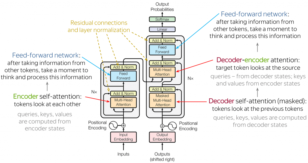
• The transformer architecture eliminates RNNs entirely, using attention both within the encoder and decoder and for interactions between them. This design enables the model to process the entire sequence simultaneously at every level.

The transformer model, therefore, represents a paradigm shift in natural language processing (NLP), offering significant improvements in speed and accuracy over RNN-based approaches.

Self-Attention

At the heart of the transformer model lies the self-attention mechanism, which facilitates efficient representation learning by enabling tokens within a sequence to interact directly with one another. Unlike traditional attention that focuses on interactions between the encoder and decoder, self-attention operates within a single representation, such as all encoder states in a particular layer.

This mechanism relies on three key components: Query (), Key (), and Value (). Each token in the sequence generates these components:

• The Query represents the information a token seeks.
• The Key identifies the information each token can provide.
• The Value contains the actual information that can be shared.

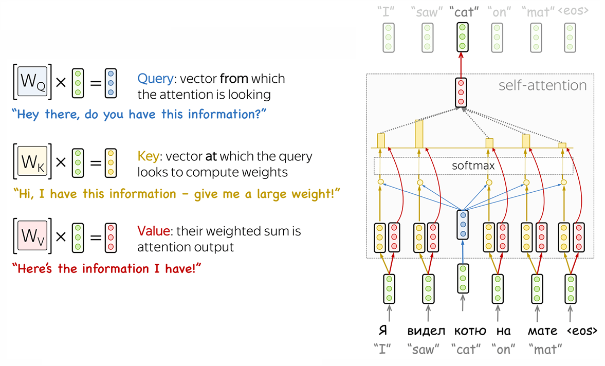
The self-attention mechanism computes the relationship between tokens by evaluating the similarity between the and vectors. This similarity is used to weight the vectors, effectively capturing how much attention each token should pay to every other token in the sequence.

Self-Attention

The formula for self-attention is given by:

where, is the dimensionality of the and vectors, and the softmax operation ensures that the attention weights sum to 1, representing a probability distribution over the tokens.

The use of , , and enables parallel computation across all tokens, making training significantly faster compared to sequential RNNs.

Multi-Head Attention

In language processing, different words may play multiple roles simultaneously. For instance:

• A verb might need to agree with its subject in gender and number.
• An object might need to be inflected based on the case determined by the verb.

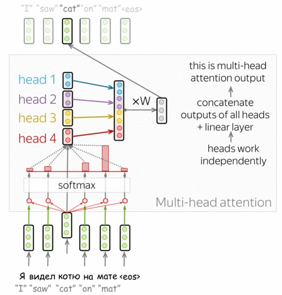
To address these varied dependencies, transformers use multi-head attention. This mechanism allows the model to learn multiple representations of the sequence by dividing the input into several attention “heads.” Each head focuses on a different aspect of the input sequence. The outputs of all heads are concatenated and transformed into a unified representation.

Multi-Head Attention

The multi-head attention mechanism is defined mathematically as:

where each attention head is computed as:

where, , , and are learned projection matrices for the , , and for head , while projects the concatenated heads into the final output space. Importantly, this design ensures that the model size remains constant regardless of the number of heads, maintaining computational efficiency.

Masked Self-Attention

The attention mechanism in the decoder operates differently during training and inference, reflecting the distinct requirements of these two phases. At inference time, tokens are generated sequentially, one at a time. This process ensures that the model does not have access to future tokens in the sequence, as their existence is not yet determined. Consequently, there is no “look-ahead” issue during inference; the model computes attention based only on the tokens generated up to that point.

In contrast, training time introduces a unique challenge. Since the entire output sequence is already known, it would be computationally efficient to process all tokens in parallel. However, this creates a “look-ahead” problem, as the model might inadvertently use future tokens to predict earlier ones. To address this, a masking mechanism is employed. This mask prevents attention from accessing information about tokens that lie beyond the current decoding step. This ensures that the model mimics the sequential generation process of inference, even when processing sequences in parallel.

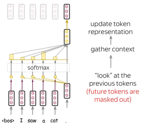
The efficiency of these mechanisms highlights a key difference between traditional RNNs and transformers:

• RNN Training scales linearly with the lengths of the source and target sequences, requiring time.
• Transformer Training, on the other hand, benefits from parallelization and operates in constant time with respect to the length of fixed sequences, significantly accelerating training on large datasets.

Building Blocks of Efficiency

The transformer architecture owes its remarkable performance not only to attention mechanisms but also to several carefully designed components:

Feedforward Networks

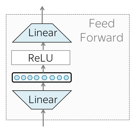
Each transformer layer contains a feedforward block consisting of two fully connected layers with a non-linear ReLU activation function in between. This block operates independently on each position of the sequence, enabling efficient processing. Mathematically, it can be expressed as:

where, and are weight matrices, while and are biases. The feedforward network enhances the transformer’s capacity to model complex patterns by introducing non-linear transformations.

Layer Normalization

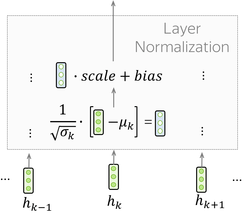
To stabilize training and improve convergence, transformers employ layer normalization. Unlike batch normalization, which operates across features for all examples in a batch, layer normalization normalizes each vector representation independently. This process ensures that the input to each layer has a mean of zero and a standard deviation of one. Additionally, trainable scale and bias parameters allow the model to learn optimal normalization dynamics for each layer.

Residual Connections

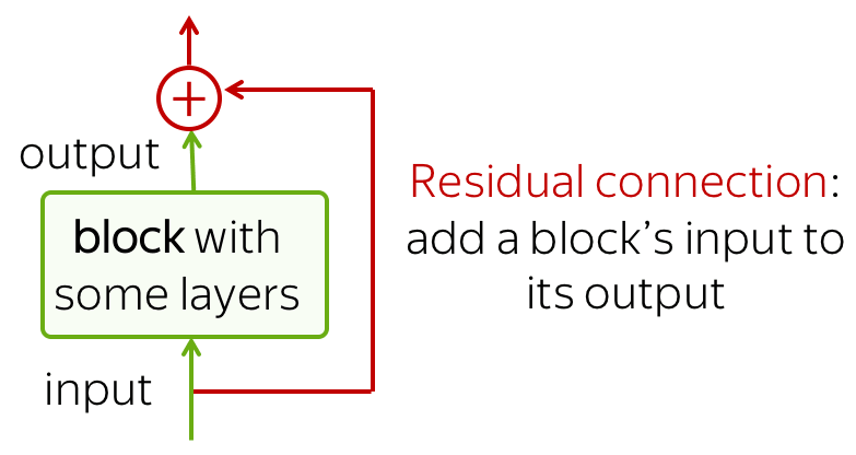
Transformers also include residual connections that add the input of each layer to its output. These skip connections facilitate the flow of gradients during backpropagation, mitigating the vanishing gradient problem and improving the training of deep architectures. They also allow layers to refine the representations incrementally, rather than starting from scratch.

The Challenge of Permutation Invariance in Self-Attention

The self-attention mechanism in transformers is inherently permutation-invariant. This means that it treats all tokens as an unordered set, focusing only on their content rather than their position in the sequence. While this property is beneficial for certain tasks, it can pose challenges in sequence modeling, where word order is crucial for understanding meaning.

Example

For example, the sentences “The cat chased the mouse” and “The mouse chased the cat” contain the same tokens but convey entirely different meanings due to their word order.

To address this limitation, transformers use positional encoding to inject information about the position of each token in the sequence. Positional encodings are added to the input embeddings, enabling the model to differentiate between tokens based on their order. These encodings are designed to be learnable or predefined using sinusoidal functions, which provide a continuous and unique representation for each position.

Positional Encoding in Transformers

In the transformer model, the representation of each input token is augmented with positional information to account for the sequential nature of language. Unlike recurrent neural networks (RNNs), transformers lack an inherent sense of order due to their parallel processing capabilities. To address this, the transformer encodes positional information as a separate embedding, which is combined with the token embeddings.

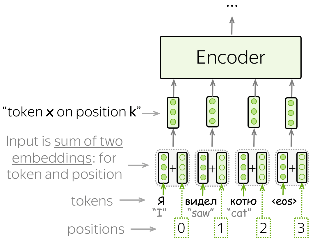
Specifically, the input representation for each token is the sum of two components:

1. The token embedding, which encodes the token’s semantic meaning.
2. The positional embedding, which encodes the position of the token in the sequence.

The original transformer model employs fixed positional encodings, although learned embeddings have also been explored. Experimental results have shown that learned positional embeddings do not significantly improve performance compared to fixed encodings.

The Mathematical Formulation of Fixed Positional Encodings

The fixed positional encodings are derived using sinusoidal functions, specifically sine and cosine, applied at varying frequencies. This approach creates a unique pattern for each position in the sequence. The encoding for position in dimension is given by:

where:

• is the position of the token in the sequence.
• is the dimension index of the embedding.
• represents the dimensionality of the token embedding vector.

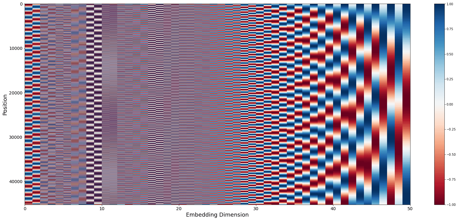
By alternating sine and cosine functions across dimensions, the encoding ensures that each position is mapped to a unique vector while maintaining continuous patterns across dimensions. This continuity enables the model to recognize relative positions and distances between tokens in the sequence.

Intuition Behind Sinusoidal Positional Encodings

The choice of sinusoidal functions for positional encodings is rooted in their periodic nature and their ability to represent positional information as patterns of alternating frequencies. These frequencies decay exponentially as the dimensions increase, ensuring that different dimensions capture different aspects of positional variation. This design has several advantages:

• Relative Positioning: The model can easily compute relative positions of tokens by learning simple linear transformations of these encodings. For example, given two positions and , their encodings and exhibit predictable phase differences that the model can exploit.
• Alternating Bit-Like Patterns: The encodings resemble alternating binary bits, where lower-frequency dimensions capture fine-grained positional changes, and higher-frequency dimensions represent broader patterns.

The sinusoidal approach provides a continuous and smooth encoding space, which is beneficial for tasks requiring precise relative positioning of tokens.

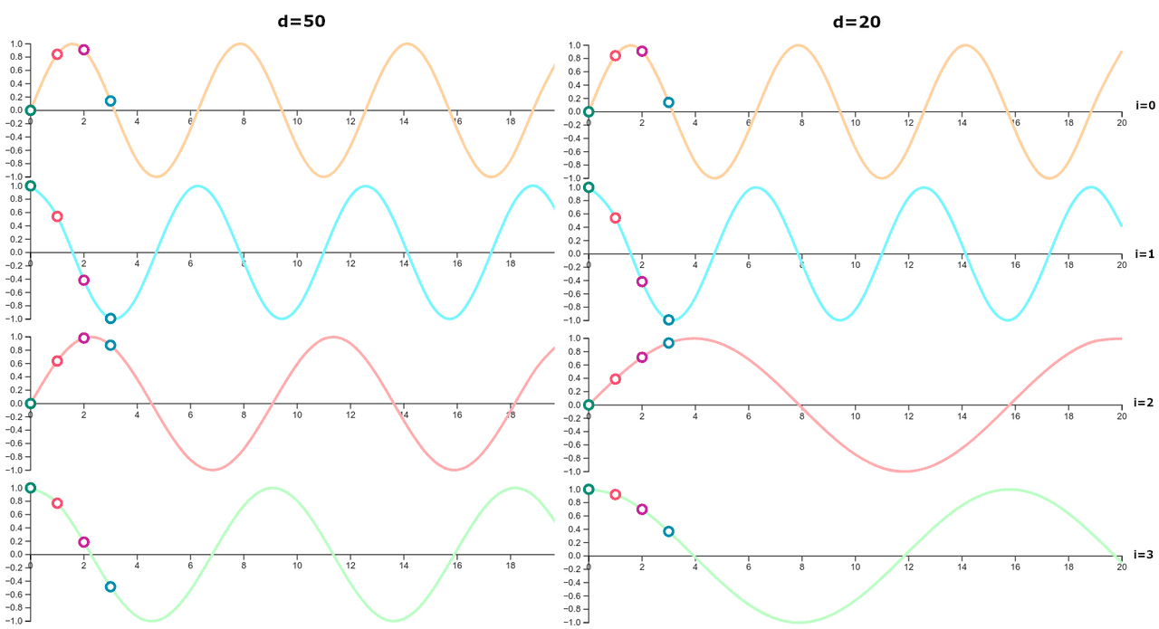
The sinusoidal patterns of positional encodings can be visualized as oscillations that alternate between high and low values across the sequence. This design mirrors the alternating behavior of binary bits, where:

• The least significant bit alternates with every position.
• Higher bits alternate less frequently, halving their frequency with each successive bit.

This mechanism ensures that positional encodings can capture both local and global patterns in the sequence. The authors of the transformer hypothesized that these sinusoidal functions would facilitate the model’s ability to attend to tokens based on relative positions, as any fixed offset between positions can be represented as a linear transformation of the positional encodings.

Position Encoding and Relative Positioning in Transformers

In transformers, the sine-cosine positional encoding scheme is both elegant and functional. It encodes the position of tokens in a sequence using sinusoidal functions at different frequencies, enabling the model to recognize relationships between tokens based on their relative positions. To formalize this idea, we can define a transformation matrix that allows a positional encoding at position to be transformed into its equivalent at , effectively encoding relative positioning.

This transformation leverages the periodic nature of sine and cosine functions. For a given frequency , the goal is to identify a linear transformation matrix such that the following equation holds:

The matrix essentially rotates the sine-cosine pair corresponding to position by an offset , allowing the model to encode relative positional relationships.

The derivation of starts with the addition formulas for sine and cosine, which express trigonometric functions of a sum in terms of individual angles. Substituting these formulas into the desired transformation equation, we get:

By comparing terms, we derive a system of equations for the entries of :

Solving this system yields the coefficients:

Thus, the transformation matrix is explicitly defined as:

This matrix represents a rotation transformation, as it depends only on the offset and is independent of the absolute position . The rotation ensures that relative positioning between tokens is preserved and efficiently encoded.

Fixed vs. Learned Positional Encodings

While the fixed positional encoding scheme provides an effective mechanism for encoding relative positions in sequences, many state-of-the-art transformer models, such as BERT, RoBERTa, and GPT-2, adopt learned positional embeddings. Unlike fixed encodings, learned embeddings treat positional information as trainable parameters, allowing the model to optimize these representations for the specific task at hand.

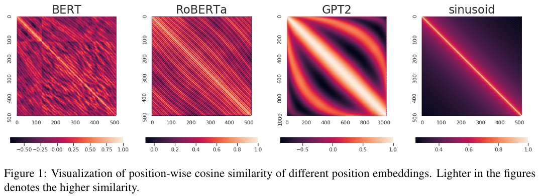
Different approaches to incorporating positional information have been explored:

1. Summation: Token embeddings and positional embeddings are summed element-wise, as in the original transformer model.
2. Concatenation: Positional information is concatenated to the token embedding vector, providing a more explicit representation of positions.

The choice between fixed and learned encodings often depends on the trade-off between interpretability (favored by fixed encodings) and task-specific adaptability (enabled by learned encodings).

Transformer Complexity and Performance Analysis

The transformer architecture is celebrated for its remarkable efficiency and ability to handle long-range dependencies in sequential data, outperforming other models such as recurrent and convolutional networks in several key aspects. A detailed comparison of their computational complexity, sequential operations, and path lengths provides insights into why transformers excel in various natural language processing tasks.

Comparison of Computational Complexity Across Layers

Layer Type	Complexity per Layer	Sequential Operations	Maximum Path Lenght
Self Attention
Recurrent
Convolutional
Self-Attention (restricted)

The complexity of each layer type in the transformer architecture is driven by its design principles:

• Self-Attention Layers:
  The computational complexity of self-attention is , where is the sequence length and is the dimensionality of the model. Despite its quadratic dependency on , self-attention enables sequential operations and achieves a maximum path length of . This unique ability to capture long-range dependencies in a single step contributes significantly to the model’s efficiency and power.

• Recurrent Layers:
  Recurrent neural networks (RNNs) have a computational complexity of , requiring sequential operations to process an input sequence. Their maximum path length is also , reflecting their stepwise dependency on prior tokens, which limits their ability to capture global dependencies efficiently.

• Convolutional Layers:
  Convolutional neural networks (CNNs) exhibit a complexity of , where is the kernel size. While they enable parallel computation, their maximum path length is , indicating that larger kernels are needed to model long-range dependencies, increasing the computational cost.

• Restricted Self-Attention Layers:
  To address the quadratic complexity of full self-attention, restricted attention mechanisms limit computations to a neighborhood of size . This reduces complexity to , while still achieving sequential operations. However, the maximum path length becomes , as the reduced attention span necessitates additional steps to capture dependencies across the sequence.

Transformers shine in scenarios where , as their self-attention mechanism becomes computationally cheaper than recurrent layers while maintaining the ability to model long-range dependencies efficiently.

Transformer Heads and Their Interpretability

An intriguing aspect of transformer models lies in the interpretability of their attention heads. These heads, which represent parallel attention mechanisms, often specialize in different tasks during training. Research has revealed that only a small subset of heads contributes significantly to the model’s performance, with others playing secondary or redundant roles. These specialized heads include:

1. Positional Heads:
   These heads focus on a token’s immediate neighbors, attending to the preceding and following tokens. Typically, 2–3 heads track previous tokens, while another 2 focus on subsequent ones. This positional awareness is vital for capturing local dependencies within a sequence.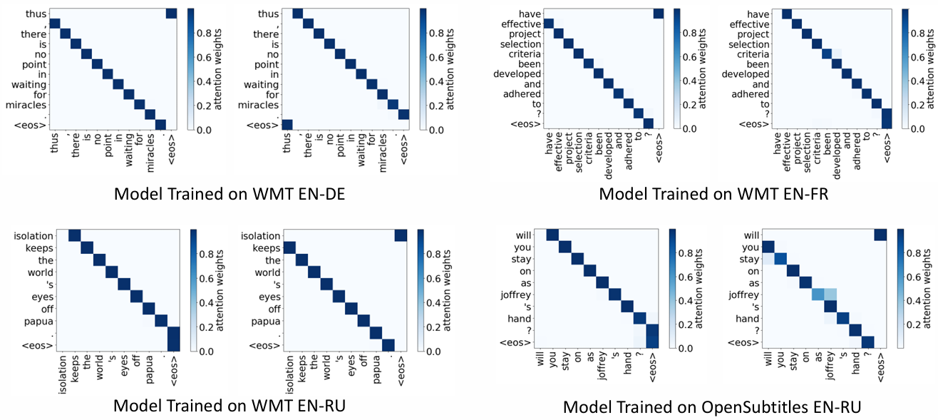

2. Syntactic Heads:
   Some heads learn to track major syntactic relations, such as subject-verb or verb-object dependencies. These heads contribute to the model’s understanding of sentence structure, improving its linguistic capabilities.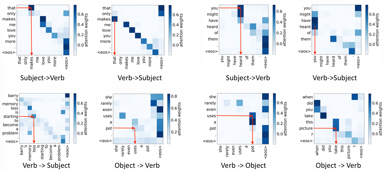

3. Rare Token Heads:
   Certain heads specialize in attending to rare tokens, particularly in the first layer. This behavior has been observed consistently across models trained on different language pairs, highlighting their importance in handling low-frequency words effectively.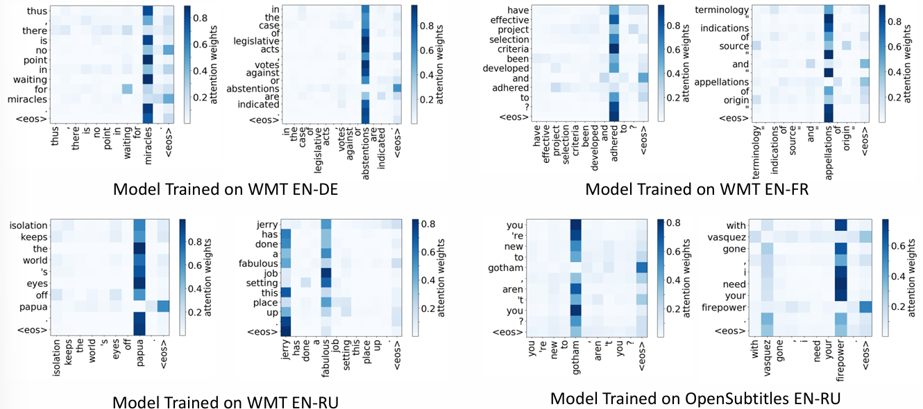

The redundancy among other heads allows for pruning, where less significant heads can be removed without significantly degrading model performance. This optimization is valuable for reducing the computational footprint of large models.

Limits of Transformers

While transformers have set new benchmarks in tasks like English-to-German (EN-DE) and English-to-French (EN-FR) translation, they are not without limitations:

1. Quadratic Complexity of Self-Attention:
   The complexity of self-attention poses challenges for very long sequences. Efforts to mitigate this, such as restricted attention or sparse attention mechanisms, involve trade-offs in capturing global dependencies.

2. Memory and Computational Demands:
   Transformers require substantial memory and computational resources, especially for large-scale models like GPT-3 or BERT. This restricts their applicability in resource-constrained environments.

3. Data Efficiency:
   Transformers often demand vast amounts of labeled data for training. While transfer learning mitigates this to some extent, low-resource tasks remain challenging.

4. Interpretability Beyond Attention:
   While attention mechanisms are interpretable to some degree, the overall behavior of transformers remains a “black box.” Understanding how they encode and utilize contextual information is an active area of research.

---

References

• Elena Voita’s NLP Course
• Text classification with Transformer
• English-to-Spanish translation with a sequence-to-sequence Transformer
• Neural machine translation with a Transformer and Keras
• The Annotated Transformer
• The Unreasonable Effectiveness of Recurrent Neural Networks
• Sequence to sequence learning with Neural networks
• Neural Machine Translation by Jointly Learning to Align and Translate
• Effective Approaches to Attention-based Neural Machine Translation
• A Neural Conversational Model
• Hierarchical Recurrent Attention Network for Response Generation
• Transformer: A Novel Neural Network Architecture for Language Understanding
• Attention Is All You Need
• The Illustrated Transformer
• Transformer Architecture: The Positional Encoding
• Positional encoding visualization
• Linear Relationships in the Transformer’s Positional Encoding
• What Do Position Embeddings Learn? An Empirical Study of Pre-Trained Language Model Positional Encoding
• Analyzing Multi-Head Self-Attention: Specialized Heads Do the Heavy Lifting, the Rest Can Be Pruned
• AI and Memory Wall