8 - Project Management

---

A project can be understood as a temporary organization established to achieve a specific goal by delivering one or more business products. According to the PRINCE2 methodology, a project is defined as

Definition

a temporary organization created for the purpose of delivering one or more business products (scope) according to an agreed Business Case (scope, cost, time, quality, risks).

This definition highlights the key characteristics of a project: its limited timeframe, the allocation of specific resources, and its focus on fulfilling clearly defined objectives within agreed constraints.

In the context of Project Management, the Project Management Body of Knowledge (PMBOK) identifies several critical variables that must be controlled to ensure the success of any project. These variables include scope, quality, schedule (time), budget (cost), resources, and risks. Project management involves systematically managing these variables through processes of planning, monitoring, and controlling to achieve the project’s objectives. Importantly, while effective management does not guarantee success, poor management almost certainly results in failure.

A simplified framework of project management often seeks to address these core questions:

1. What problem are you solving? This question determines the project’s scope.
2. How will you solve this problem? This requires defining the project strategy.
3. What is your plan? This includes detailing the work to be done, estimating its duration, identifying required resources and costs, and planning how communication, risks, quality, and changes will be managed.
4. How will you know when the project is complete? Success criteria need to be defined to evaluate when the project goals have been met.
5. How well did the project perform? After completion, an assessment of the success criteria helps gauge the project’s overall success.

Steps

The PMBOK project management process breaks down a project into five distinct phases:

1. Initiating - Defining the project’s purpose, objectives, and stakeholders.
2. Planning - Detailing the scope, schedule, costs, resources, risks, and communication mechanisms.
3. Executing - Carrying out the tasks defined in the project plan.
4. Monitoring and Controlling - Ensuring the project stays on track, managing changes, and addressing issues.
5. Closing - Finalizing all activities, handing over deliverables, and assessing outcomes.

Software Project Management

In software development, project management plays a crucial role in delivering the right product on time and within budget. Successful software organizations depend heavily on their ability to manage projects efficiently, ensuring the alignment of product delivery with business needs and constraints.

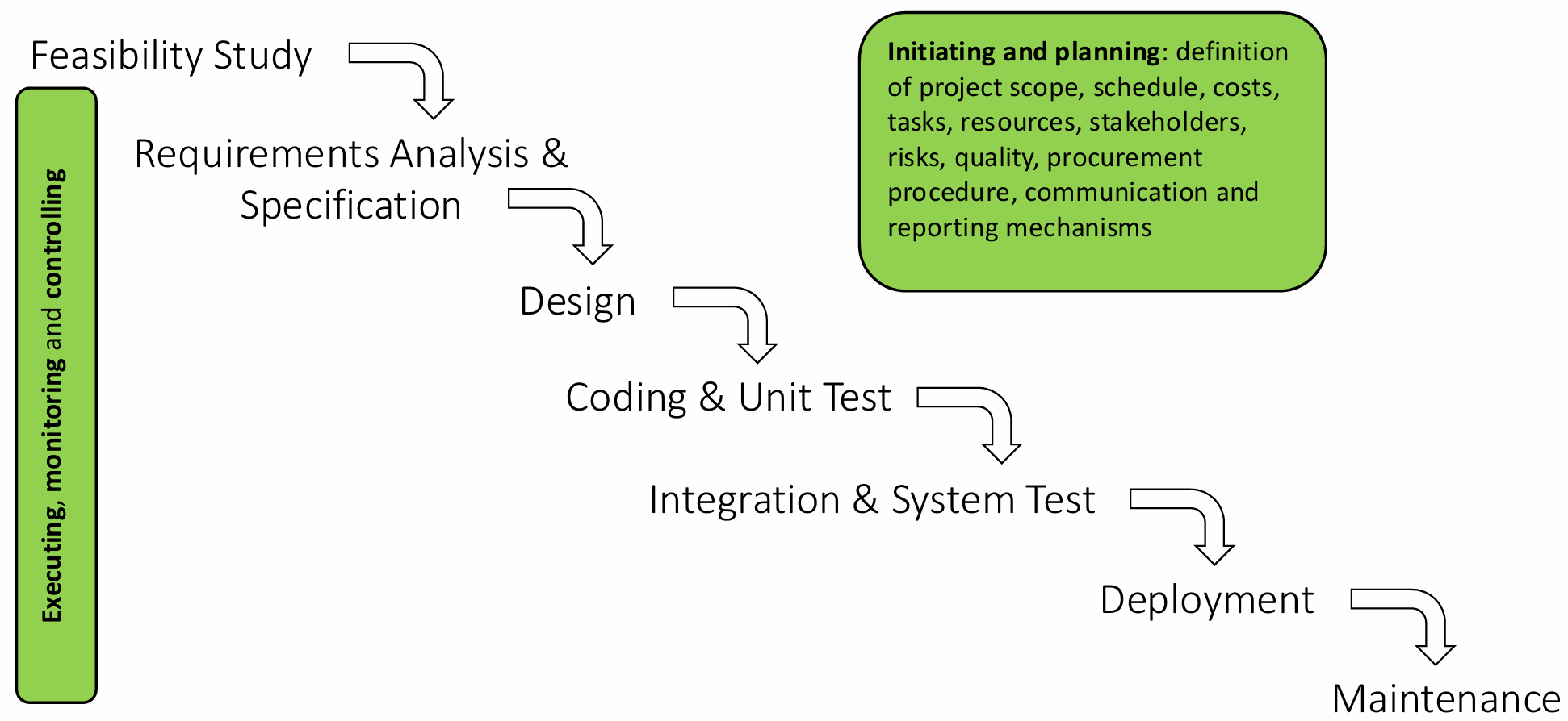
A structured software development lifecycle (SDLC) often involves the following phases:

1. Feasibility Study - Determining whether the project is viable and worth pursuing.
2. Requirements Analysis and Specification - Defining the functionality and constraints of the software product.
3. Design - Creating a technical blueprint for the system.
4. Coding and Unit Testing - Developing the software and testing individual components.
5. Integration and System Testing - Combining components and testing the entire system for functionality and performance.
6. Deployment - Delivering the software to users.
7. Maintenance - Addressing issues and updating the software as required.

Project management practices within software development encompass initiating and planning, which include defining the project’s scope, schedule, costs, resources, stakeholders, risks, quality, procurement procedures, and communication strategies. During execution, monitoring and controlling processes are applied to track progress, address deviations, and ensure that the project objectives are met.

Delays and Failures

Delays and failures in software projects are common due to the complexity of managing diverse factors such as technology, people, and changing requirements.

Example

A notable example is the troubled launch of Healthcare.gov, the website associated with the Affordable Care Act (ACA), commonly known as “Obamacare.”

The ACA, enacted in 2010, required the creation of health benefit websites to allow individuals to compare and purchase health insurance plans. States could either join the federal platform (Healthcare.gov) or build their own. A majority chose to use the federal system, placing immense pressure on its development and testing.

When Healthcare.gov was launched on October 1, 2013, it faced widespread technical issues, including slow response times, system crashes, and user errors. The complexity of integrating multiple systems, inadequate testing, and insufficient planning contributed to its failure at launch. The situation was humorously criticized by Jon Stewart, who quipped, “I’m going to try and download every movie ever made, and you’re going to try to sign up for Obamacare, and we’ll see which happens first.”

The Healthcare.gov case highlights critical lessons in project management:

1. Scope Definition - Clearly understanding and managing the scope of work is essential to avoid overcomplication.
2. Planning and Testing - Comprehensive testing and realistic timelines are crucial for system reliability.
3. Risk Management - Identifying potential risks and implementing contingency plans can mitigate unexpected issues.
4. Stakeholder Communication - Consistent and transparent communication ensures alignment across teams.

Effective project management remains a cornerstone of successful software projects. By addressing scope, quality, schedule, cost, risks, and communication systematically, organizations can navigate the complexities of project delivery and reduce the likelihood of failure.

The launch of Healthcare.gov on October 1, 2013, was marked by significant technical and operational failures. The issues observed on the first day included:

1. High Website Demand
   The website faced five times the expected user load, with 250,000 users accessing it within the first two hours. This unexpected demand caused the system to crash and become inaccessible for most users.

2. Incomplete Design and Implementation
   Critical parts of the website were not fully developed at the time of launch:

   • Drop-down menus and navigation features were incomplete.
   • Sensitive user data was transmitted over insecure HTTP connections, exposing users to privacy risks.

3. Login Feature Bottleneck
   The login functionality, a key feature, was unable to handle high traffic. Even system administrators relied on this login feature, preventing them from intervening effectively during the crisis.

4. Poor User Outcomes
   On launch day, only six users were able to complete the application process, select a healthcare plan, and successfully submit their information.

These shortcomings reflected systemic issues in planning, execution, and testing. Despite the disastrous start, Healthcare.gov saw substantial improvements over the following weeks:

1. Enhanced Technical Capacity
   New contractors and improved management practices enabled the system to handle 35,000 concurrent users by December 1, 2013.

2. Successful Enrollment
   By December 28, the end of the open enrollment period, 1.2 million users had successfully signed up for healthcare plans.

These improvements highlight the importance of addressing core technical and management failures promptly to restore functionality and trust.

A post-mortem analysis of the failure revealed multiple underlying causes:

1. Lack of Relevant Experience
   Project managers overseeing Healthcare.gov lacked the necessary expertise in software development processes. Their limited understanding of best practices for building and launching complex digital systems contributed to the system’s instability.

2. Leadership and Communication Failures
   Poor coordination among various government offices and contractors led to unclear division of responsibilities. For example, low resource allocation for the login feature was based on the assumption that users would log in only after selecting their desired healthcare plan. This assumption was later changed, but the change was not communicated effectively, leading to bottlenecks.

3. Schedule Pressure
   The launch date was fixed due to political and legal deadlines, regardless of whether the system had undergone sufficient testing. The rushed schedule left little time to debug critical issues.

4. Cost Overruns
   The project was initially budgeted at 1.7 billion. This dramatic increase reflected inefficiencies in both planning and execution.

Initiating and Planning Process

The issues faced by Healthcare.gov underscore the importance of robust initiating and planning processes in project management:

1. Initiating
   This phase focuses on securing a commitment to start the project. It includes: clearly defining the project’s scope and strategy to ensure alignment among stakeholders.

2. Planning
   Detailed planning lays the groundwork for successful execution, monitoring, and controlling. Key activities include:

   • Defining the project schedule to establish realistic timelines.
   • Identifying stakeholders and assessing potential risks.
   • Estimating costs and allocating resources effectively.
   • Establishing processes for:
     • Communication: Deciding when and how information will be shared.
     • Procurement: Managing how external resources and services will be acquired.
     • Monitoring and Control: Setting up mechanisms to track progress and make necessary adjustments.

Lessons Learned

The Healthcare.gov case serves as a cautionary tale for managing large-scale projects. It demonstrates the need for:

• Technical Expertise: Assigning knowledgeable project managers who understand the intricacies of software development.
• Clear Communication: Ensuring seamless coordination among all stakeholders and contractors.
• Adequate Testing: Allocating sufficient time for testing and debugging before launch.
• Realistic Planning: Balancing political or external deadlines with the project’s technical readiness.

By prioritizing these elements, future projects can avoid similar pitfalls and ensure a smoother path to success.

Project scheduling is a fundamental aspect of project management, encompassing the planning and organization of tasks, milestones, and deliverables to achieve project goals within a defined timeframe. Proper scheduling ensures efficient resource allocation, identifies potential bottlenecks, and tracks progress toward completion.

Definition

1. Tasks
   Tasks, also known as Work Packages (WPs), are specific activities that need to be completed to accomplish the project’s goals. Tasks are often defined at a granular level to simplify estimation, assignment, and monitoring.

2. Milestones
   Milestones are significant points in the project timeline where progress can be evaluated. For example, the delivery of a system for testing or the completion of coding. These serve as checkpoints to ensure the project stays on track.

3. Deliverables
   Deliverables are the tangible work products delivered to the customer, such as components of the software solution or final documentation.

Planning the Project Schedule

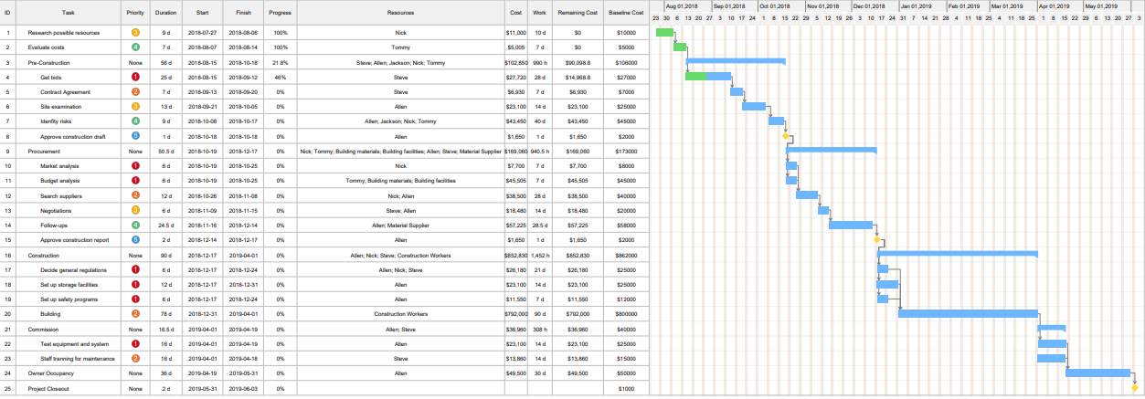
Graphical tools are widely employed to visualize project schedules. Among these, Gantt charts are the most common, presenting a timeline where activities or resources are mapped against time.

Definition

A Gantt chart provides a visual representation of tasks, their durations, and their sequence. It is particularly useful for tracking progress and identifying dependencies.

Techniques for Creating Project Schedules

Several methodologies are used to design project schedules. These include:

1. Work Breakdown Structure (WBS)
   WBS decomposes the project into smaller, manageable tasks, enabling better estimation, assignment, and monitoring. Each level of the WBS adds more detail, as shown below:
   

2. Precedence Diagram Method (PDM)
   PDM focuses on defining dependencies between tasks:

   • Finish-to-Start (FS): The successor cannot begin until the predecessor finishes.
   • Start-to-Start (SS): The successor can start once the predecessor starts.
   • Finish-to-Finish (FF): The successor finishes only when the predecessor finishes.
   • Start-to-Finish (SF): The successor cannot finish until the predecessor starts.
     Lags, positive or negative delays between tasks, can also be introduced to account for specific requirements.

3. Critical Path Method (CPM)
   CPM identifies the sequence of tasks that directly impact the project completion date. Tasks along the critical path have zero float, meaning any delay in these tasks will delay the entire project. Key elements include:

   • Calculating early start (ES), early finish (EF), late start (LS), and late finish (LF) for tasks.
   • Highlighting critical tasks and optimizing their execution to avoid delays.

Task constraints influence when tasks can start or finish:

• Flexible Constraints: Tasks start as early as possible.
• Partially Flexible Constraints: Tasks have specific conditions, such as “not starting earlier than” or “finishing no later than.”
• Inflexible Constraints: Tasks occur on fixed dates, often due to external dependencies.

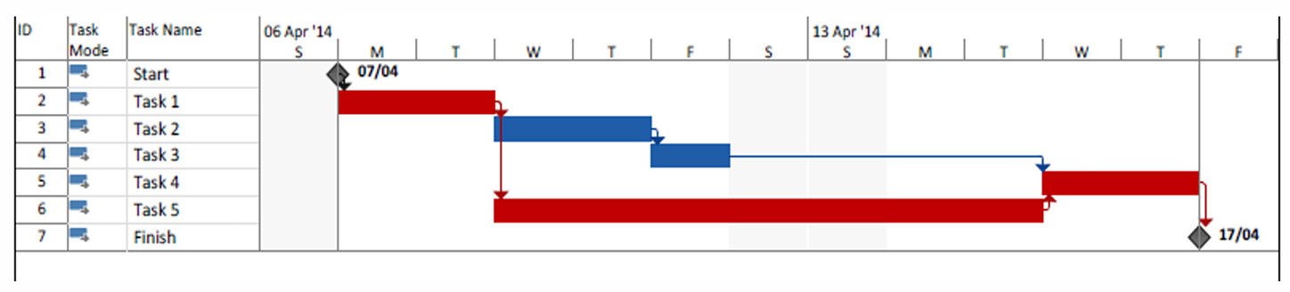
Example: Critical Path Analysis

Consider the following project schedule network:

• Critical Path: T1 → T5 → T4
  
• Duration: 9 days (minimum time required to complete the project).
• Tasks not on the critical path, such as T2 and T3, have a float, allowing flexibility in scheduling without impacting the project’s finish date.

Risk Management Plan

Risk management is a structured process to identify, analyze, address, and monitor risks throughout a project’s lifecycle. Its primary objective is to establish a framework that allows for proactive handling of potential threats to ensure project goals are met.

Definition

A risk refers to a potential problem or threat that could negatively impact a project.

Identifying risks involves uncovering potential threats to the project using several approaches:

1. Prior Experience: Leveraging insights gained from previous projects.
2. Brainstorming: Engaging the team and stakeholders to uncover possible risks.
3. Lessons Learned: Applying knowledge from similar projects.
4. Checklists: Using predefined lists of common risks in similar domains.

A practical rule of thumb when formulating risks is to use the structure:

This ensures that the risk is explicitly linked to its cause, impact, and the stakeholder affected.

A correct risk formulation clearly identifies the situation, consequence, and stakeholder. For example, “If data storage tools are inadequate, then significant response time delays can occur for end users.” This structure ensures that the risk is explicitly linked to its cause, impact, and the stakeholder affected, making it easier to understand and address.

In contrast, an incorrect risk formulation is missing one or more elements, such as a stakeholder or a properly defined situation. This leads to a poorly understood cause-effect relationship, making it difficult to assess and mitigate the risk effectively. For instance, a statement with a consequence but no stakeholder does not clearly indicate the impact on the project, while a consequence without a situation does not properly explain the cause, requiring further analysis.

Examples of Risk Statements

1. If functional requirements are not fully met, then user dissatisfaction may arise, for project stakeholders.
2. If functional requirements are not well understood, then implementation delays may occur, for the development team.

Once risks are identified, they must be evaluated based on two critical factors:

1. Likelihood: The probability that the risk will materialize, expressed as a percentage or qualitative level (e.g., low, medium, high).
2. Impact: The degree of damage the risk could cause, which may include financial loss, performance degradation, or reputational harm.

NASA uses a 5x5 risk matrix to visualize and prioritize risks. This matrix categorizes risks based on:

• Probability: Five levels ranging from very low to very high.
• Impact: Five levels representing the severity of consequences, from negligible to catastrophic.

Each risk is plotted based on its likelihood and impact, helping project managers focus on high-probability, high-impact risks first.

Exercise: reformulate and re-evaluate the risks in a correct way

Risk	Probability	Impact
Organizational financial problems force reductions in the project budget	Low	Catastrophic
It is impossible to recruit staff with the skills required for the project	High	Catastrophic
Key staff are ill at critical times in the project	Moderate	Serious
Faults in reusable components must be repaired before these components are reused	Moderate	Serious
Changes to requirements that require major design rework are proposed	Moderate	Serious

The risk register example

Risk	Probability	Impact	Mitigation Strategy
If in the project budget, organizational financial problems arise, then they will force reductions b the project team.	Unlikely	Catastrophic	Reduce project scope and revise requirements accordingly
If the labour market lacks candidates with the skills required for the project, then this will cause a reduction in the team workforce, for the project team.	Very likely	Critical	Plan for training available staff
If key staff is sick at critical times in the project, then this determines that the project is delayed, for the project team.	Likely	Moderate	Assign more than one staff member to critical components so that it is less likely that all of them are sick at the same time
If reusable software components show defects, then this causes delays in the project, for the project team.	Likely	Moderate	Plan for careful testing and bug fixing for these reusable components before their usage
If changes in requirements that require major design rework are proposed, then this determines the need for an extra effort, for the project team.	Likely	Moderate	Identify the involved components, replan for a new development iteration to address these changes

Executing, Monitoring, and Controlling

Project execution and monitoring are critical phases in project management that ensure the planned tasks are performed effectively, tracked accurately, and adjusted as necessary to achieve project goals.

The execution phase focuses on launching and carrying out the tasks defined in the project plan. Key activities include:

1. Project Kickoff: Initiate the project with a meeting that aligns all stakeholders on goals, deliverables, and expectations.
2. Resource Management: Assemble and manage both internal and external project teams, ensuring the availability of required equipment, materials, and services.
3. Task Implementation: Execute the work as outlined in the schedule, ensuring all tasks progress according to plan.
4. Monitoring Activities: Continuously track progress and make adjustments as necessary to stay aligned with project objectives.

Projects rarely adhere strictly to initial plans due to unforeseen changes or challenges. Monitoring and controlling processes are used to ensure alignment with the project’s baseline plan by:

• Monitoring: Gathering data to understand the current status of the project.
• Controlling: Implementing corrective actions to address deviations from the plan.

These processes involve data collection, comparison against the baseline, and adjustments as required to ensure successful project delivery.

Data Gathering

Accurate and current data collection is the foundation of effective monitoring. Key areas to track include:

1. Task Progress: Start and completion dates for tasks.
2. Work Hours: Actual hours worked or task durations.
3. Remaining Work: Estimate of remaining effort to complete tasks.
4. Costs: Actual money spent compared to budgeted amounts.

This data is then used to update the project schedule, with the original plan serving as the baseline for comparison.

Monitoring Schedule and Costs

The project’s actual performance is measured against its baseline in two critical areas:

1. Schedule: Identify delays, unstarted tasks, or uncompleted work.
2. Costs: Compare actual expenses to the allocated budget.

Warning signs include tasks running late or costs exceeding projections, both of which require prompt corrective actions.

Risk Monitoring

Risks identified in the project’s risk management plan must be continuously monitored. If a risk materializes, the mitigation strategies outlined in the plan should be implemented. If those strategies prove ineffective, they may need to be revised to better address the situation.

Earned Value Analysis (EVA)

Definition

EVA is a methodology for evaluating project performance by integrating the variables of scope, time, and cost into a single, comparable financial measure.

EVA simplifies complex data, allowing project managers to identify variances and trends effectively.

Key Metrics in EVA:

1. Budget at Completion (BAC): Total project budget.
2. Planned Value (PV): Budgeted cost of work scheduled.
3. Earned Value (EV): Budgeted cost of work performed.
4. Actual Cost (AC): Actual cost incurred for completed work.

By comparing these metrics, managers can assess both cost and schedule performance.

EVA Example - OS Servers' Upgrade

Project Scope: Upgrade four servers in four weeks with a budget of €400.

Week	Scope	Budget (€)
1	Server 1	100
2	Server 2	100
3	Server 3	100
4	Server 4	100

Monitoring at the End of Week 2

At the end of the second week, the project has incurred actual costs of €150, with only one server upgraded. This is compared to the planned expenditure of €200, which was intended to cover the upgrade of two servers.

To assess the project’s performance, we conduct an Earned Value Analysis (EVA). The Earned Value (EV), which represents the budgeted cost of the work performed, is €100 for the single server upgraded. The Planned Value (PV), or the budgeted cost of the work planned, is €200 for the two servers. The Actual Cost (AC) spent is €150.

Variances and Performance

1. Schedule Variance (SV):
   The Schedule Variance is calculated as:

   A negative SV of indicates that the project is behind schedule, as less work has been completed than planned.

2. Cost Variance (CV):
   The Cost Variance is determined by:

   A negative CV of signifies that the project is over budget, as the actual costs exceed the budgeted costs for the work performed.

3. Performance Indices:

   • Schedule Performance Index (SPI):
     The SPI is calculated as:

     An SPI of , which is below , indicates poor schedule performance, meaning the project is progressing at half the planned rate.

   • Cost Performance Index (CPI):
     The CPI is computed as:

     A CPI of , also below , suggests inefficient cost management, as the project is spending more than budgeted for the work completed.

Earned Value Analysis (EVA) provides tools for predicting the Cost Estimate at Completion (EAC) based on different assumptions about spending and performance rates.

Cost Estimate at Completion (EAC)

1. Assumption 1: Continue spending at the same rate (same CPI).

2. Assumption 2: Continue spending at the baseline rate.

3. Assumption 3: Both cost and schedule performance (CPI and SPI) influence the remaining work.

EVA Example: OS Servers' Upgrade

• CPI:

• SPI:

Budget Predictions:

1. Same CPI:

2. Baseline Rate:

3. Same CPI and SPI:

These estimates demonstrate the impact of performance inefficiencies on overall project cost.

Controlling Process

Controlling involves balancing the competing priorities of scope, time, cost, resources, and quality to ensure project success. This process requires making informed decisions that align with stakeholders’ priorities while effectively managing associated risks.

Controlling Techniques

Fast Tracking involves accelerating project tasks by starting them earlier or running them in parallel. The advantage of this technique is that it does not increase costs. However, it carries a higher risk due to task dependencies and the potential for increased complexity.

Crashing involves reducing task durations on the critical path by adding resources. This technique allows for faster project completion. The downside is that it increases costs and may have limited feasibility if additional resources cannot be effectively utilized.

By carefully applying these techniques, project managers can address schedule constraints and ensure timely project delivery while balancing other project variables.

Crashing Example

The project duration is reduced from 9 days to 5.5 days at an additional cost of €1450.

Task Name	Original Duration (days)	Crash Length (days)	New Duration (days)	Crash Cost/Day (€)	Crash Cost (€)
Task 1	2	0.5	1.5	400	200
Task 4	2	1	1	250	250
Task 5	5	2	3	500	1000

Totals:

• Original Duration: 9 days
• New Duration: 5.5 days
• Total Crash Cost: €1450

Closing Process

The project is concluded through:

1. Acceptance: Obtain stakeholder approval for deliverables.
2. Performance Tracking: Analyze outcomes against objectives.
3. Lessons Learned: Document experiences to inform future projects.
4. Contract Closure: Finalize and close all agreements.
5. Resource Release: Reassign or release team members and equipment.

Effort and Cost Estimation in Software Development

Effort and cost estimation are fundamental components in the planning and management of software development projects. These estimations help organizations allocate the right resources, manage budgets, and adhere to schedules, all of which are crucial for project success. The process involves determining the amount of work required to develop software products and deliverables, taking into account various influencing factors that may affect the overall project scope.

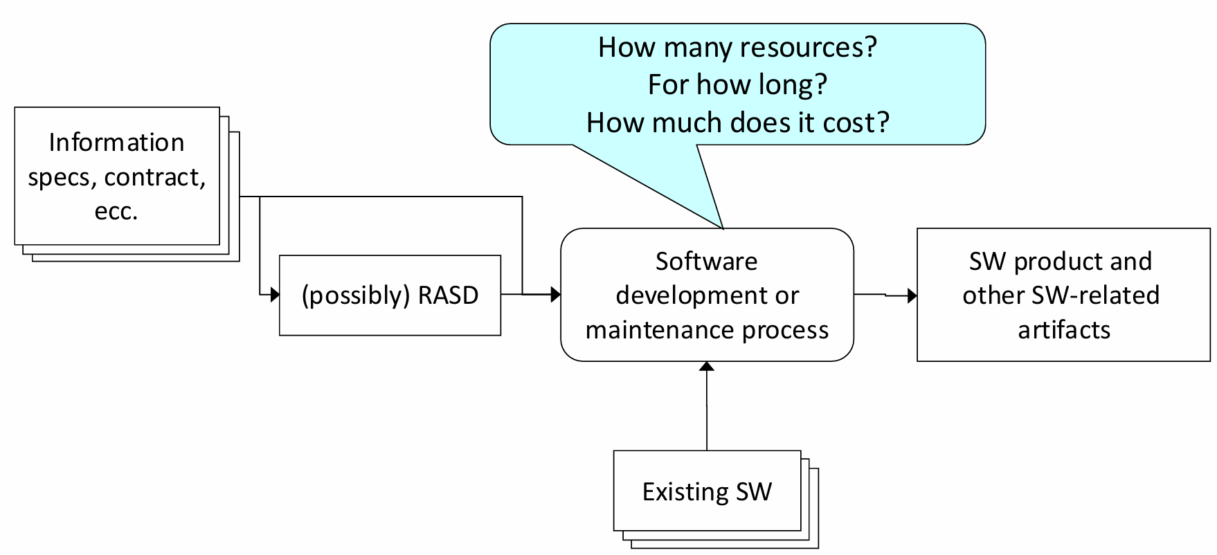
Estimating effort and cost in software development is a complex and challenging task. This complexity arises from several factors:

1. Inputs to the Estimation Process: The inputs typically consist of specifications, contracts, and in some cases, a detailed Requirements Analysis and Specification Document (RASD). These documents provide the foundational information needed to define the software requirements and deliverables.

2. Outputs of Estimation: The ultimate outputs of the estimation process include not just the software products themselves, but also related artifacts such as documentation, testing plans, and deployment strategies. These outputs are interconnected and must be considered when estimating the required effort and associated costs.

3. Interdependencies: Estimating software effort is further complicated by the interdependencies between existing software systems, project-specific requirements, and external constraints. These factors influence the development process, making it harder to generate accurate estimates, especially for projects that involve integration with legacy systems or new technologies.

Techniques for Effort and Cost Estimation

Organizations typically use two main techniques for estimating the effort and cost required for software development: experience-based techniques and algorithmic cost modeling.

Experience-Based Estimation Techniques

Experience-based estimation methods rely on the knowledge and past experience of the development team. These methods are often quicker and more intuitive, making them suitable for projects where the team has prior experience or a similar project to refer to. The process generally involves identifying the deliverables (such as documents, modules, or specific features), documenting them, and estimating the effort required for each deliverable. These individual estimates are then aggregated to form a total estimate for the project.

One key advantage of experience-based techniques is their adaptability to the specific organizational context. These methods can be tailored based on the team’s past performance and familiarity with similar projects, which can result in faster estimations for projects with known characteristics. However, the downside is that they can be highly subjective and prone to biases, especially if the project is complex or unfamiliar. The technique may also struggle to scale well for large or highly intricate projects, where historical data might not provide sufficient guidance.

Algorithmic Cost Modeling

Algorithmic cost modeling, on the other hand, uses mathematical formulas to estimate the effort required for a project. These models are based on project attributes such as size, complexity, and the experience level of the development team.

New formula

A common formula used in algorithmic models is:

In this formula:

• is an organization-dependent constant,
• represents a quantitative measure of the product, such as lines of code (LOC) or function points (FP),
• accounts for the non-linear relationship between effort and project size, and
• is a multiplier that adjusts for factors such as project complexity, team skills, and process maturity.

The primary benefit of algorithmic models is their ability to provide consistency and scalability. These models are particularly useful during the early stages of a project when high-level estimations are required. They offer a more objective approach, which can be particularly advantageous when estimating large or unfamiliar projects. However, they require accurate input parameters and can sometimes oversimplify the realities of a project, especially when dealing with highly unique or innovative tasks.

Estimation Accuracy and Factors Influencing It

Accurate effort and cost estimation is inherently challenging, especially during the early phases of a project when limited information is available. However, as the project progresses and more details are uncovered, the accuracy of the estimations generally improves.

Several factors influence the accuracy of software estimation:

1. COTS Components: The use of Commercial Off-The-Shelf (COTS) components can significantly reduce development effort. These pre-existing solutions often require less customization and integration effort compared to building components from scratch.
2. Programming Language: The choice of programming language also affects the development effort. Higher-level languages that offer abstraction from hardware or lower-level operations often result in less effort required for implementation.
3. Team Distribution: Geographically dispersed teams or teams from different cultural backgrounds may face communication challenges that could impact productivity. These factors can influence the overall effort required to complete the project.

To improve the accuracy of estimates, organizations should aim to refine their estimation processes as more information becomes available. Regular reviews and adjustments to the estimates can help account for unforeseen challenges and opportunities.

Managing Estimate Uncertainty

Due to the inherent uncertainty in software development, especially in the early stages, it is crucial to have robust procedures for estimation. Even though uncertainty is a constant, a well-structured estimation process, coupled with the use of both experience-based techniques and algorithmic models, can help improve the reliability of estimates. As the project evolves and more data becomes available, estimates should be updated to reflect new insights, thus reducing uncertainty and improving decision-making.

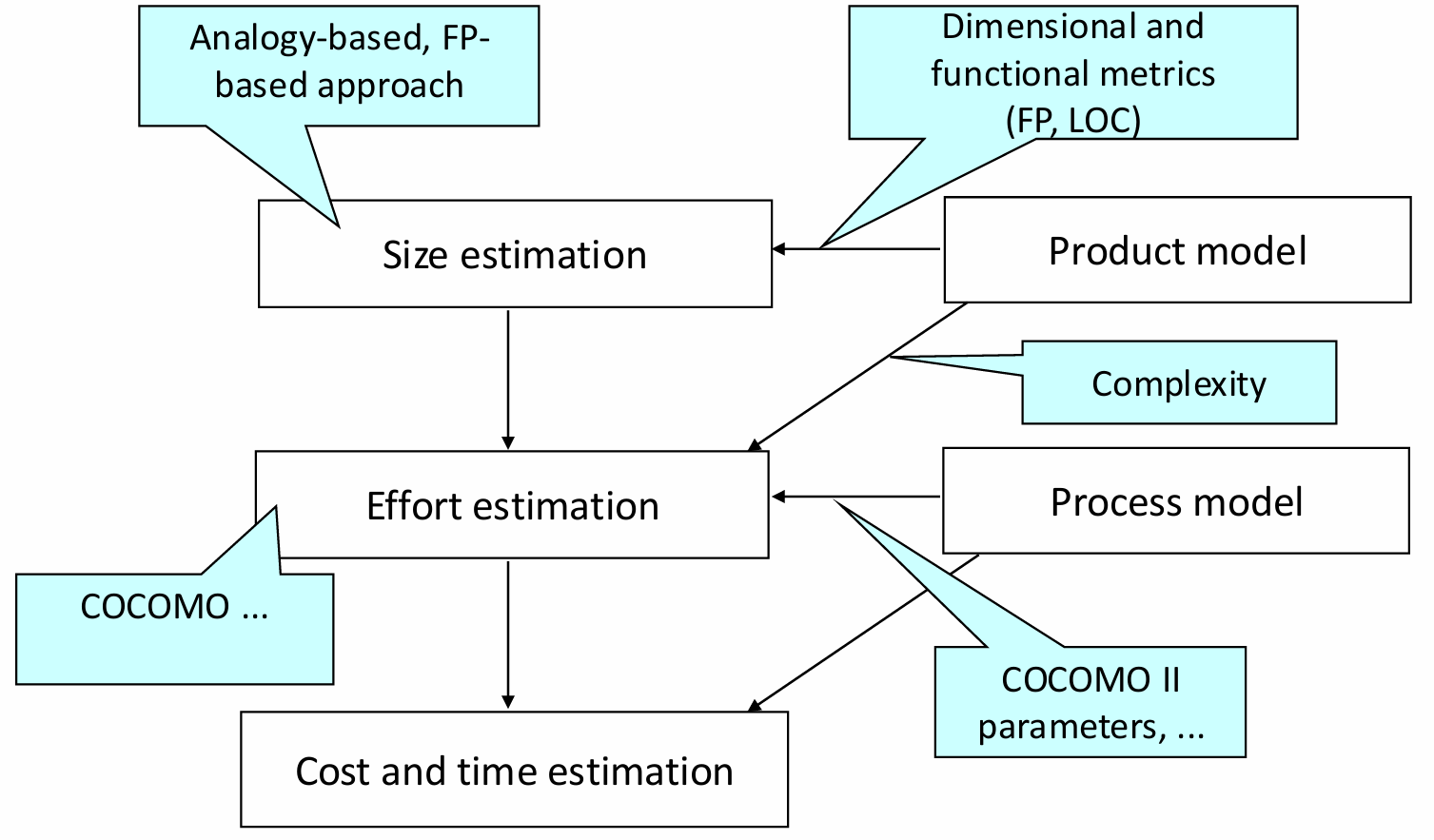
The typical estimation process involves several stages, which are designed to refine the estimates as the project progresses.

Steps

These stages include:

1. Size Estimation: The first step involves determining the expected size of the software product. This can be done using methods such as Function Points or Lines of Code (LOC), which provide an objective measure of software size. The choice of method often depends on the nature of the project and the availability of data.

2. Effort Estimation: Once the size is estimated, it is used as input for determining the effort required. This can be done through experience-based techniques or by applying an algorithmic cost model. The effort estimation typically involves factoring in various environmental and project-specific variables.

3. Cost and Time Estimation: Finally, effort estimates are translated into cost and time projections. This step typically involves using process models that account for the development process, team structure, and any external dependencies that may impact the schedule.

Estimating Software Size

Accurate estimation of software size is a crucial part of the effort estimation process. There are two primary methods for estimating software size: Function Points (FP) and Lines of Code (LOC).

• Function Points Method Function Points measure the size of software based on the functionality it provides to the user. This method, introduced by Allan Albrecht of IBM in 1975, involves analyzing the software’s features and classifying them into various function types (such as inputs, outputs, inquiries, internal files, and external interfaces). These function types are then assigned a weight based on their complexity. The total function point count is then used to estimate the size of the software product.

• Lines of Code (LOC) Estimation Alternatively, Lines of Code (LOC) is a direct method of estimating software size. This method involves estimating the total number of lines of code that will be written for the project, either through historical data or expert judgment. This estimate can be refined with a complexity analysis that accounts for particularly challenging features or high-risk areas of the software.

Definition

Function Points (FP) are a standardized unit of measurement used to estimate the size of a software system based on its functionality rather than the lines of code.

The calculation of Function Points is based on the following formula:

In this formula, the total Function Points are derived by summing up the contributions of each type of function, where each function type is weighted according to its complexity.

The primary idea behind Function Points is that the size of a software product can be determined by the number and complexity of the functions it performs, independent of the technology or language used to implement it.

To calculate Function Points, the software system is analyzed and categorized into several key components. Each component is associated with a function type that reflects its role in the system. The main components are:

1. Data Structures: These include internal and external data that the application manages or interacts with.
2. Inputs and Outputs: The data being processed or output by the system, including both external inputs and outputs.
3. Inquiries: Interactions where data is requested but without significant transformation.
4. External Interfaces: Interactions with external systems or applications that contribute to the overall functionality of the software.

Each of these components is assigned a weight based on its complexity, which allows the function point calculation to reflect the effort required for different parts of the system.

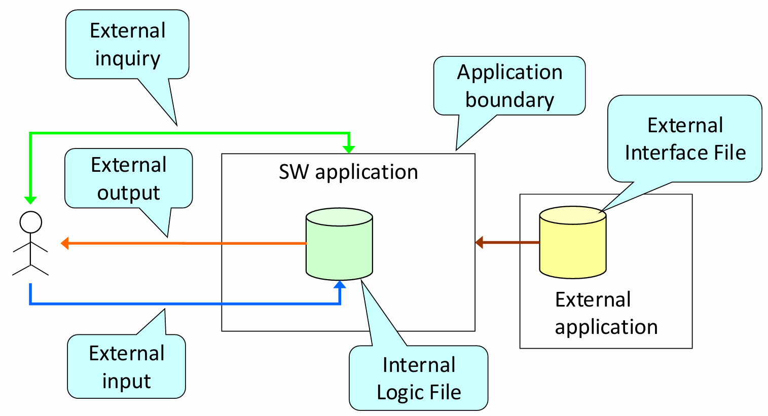
The Function Point method categorizes the functions of a software application into five core function types, each representing an aspect of the software’s external behavior. These function types are crucial for determining how complex each part of the system is and subsequently how much effort is needed for its development. The five function types are:

1. Internal Logic File (ILF): An ILF is a set of data used and managed by the application. These data elements are critical for the system’s internal functioning and represent collections of data the software handles directly.

2. External Interface File (EIF): An EIF is a set of data used by the application but maintained externally, usually by other systems. These files represent interfaces with external data sources that the software must interact with.

3. External Input: This refers to operations that receive data from external sources and process it in some way. These could be actions like form submissions, user inputs, or external system interactions that modify the system’s state.

4. External Output: These are operations that generate data for external users or systems. Outputs typically involve computation or transformation of data that is then presented to the user or forwarded to another system.

5. External Inquiry: This refers to operations where data is requested from the system but no significant processing or transformation occurs. Examples include simple queries or searches for data that do not require modification.

Historical Definition of Function Points

The concept of Function Points was originally defined by Allan Albrecht in the late 1970s, based on his analysis of 24 software applications written in languages like COBOL, PL/1, and DMS. These applications ranged in size from 3,000 to 318,000 lines of code and required between 500 and 105,200 person-hours for development. By examining these applications, Albrecht identified common patterns and relationships between software functionality and the effort required for development.

Through this analysis, Function Types were assigned weightings to reflect their relative contribution to development effort. This led to the formulation of a model that could predict the amount of effort required to develop a software system, making it a valuable tool for project estimation. The Function Points method became widely adopted as a means of estimating the size and complexity of software projects, providing a more objective measure than raw lines of code.

Function Points Calculation for a Mobile Telephony Service Application

To apply the Function Points method in a practical scenario, consider the example of a mobile telephony service application. This application handles various functionalities related to user data, rate plans, promotions, and billing. By analyzing the application’s features, we can categorize them into the five function types and calculate the total Function Points.

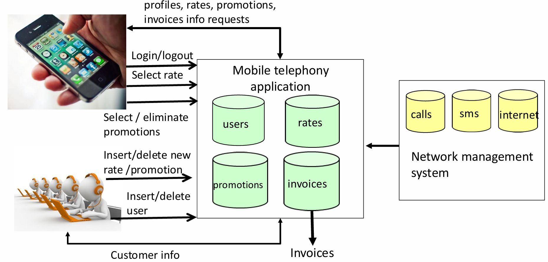
Mobile Telephony Service Application

The mobile telephony service application manages crucial data for users, such as personal information, phone numbers, subscribed rate plans, and active promotions. Each rate type within the application includes details about the costs for calls, SMS messages, and internet usage, with some rates adjusted based on promotions that apply for limited periods.

Users interact with the system to modify their details, change their rate plans, and activate or deactivate promotions. Additionally, the system integrates with an external network management system that provides data on call durations, SMS usage, internet activity, and user location during roaming. This data is used to generate billing information and ensure that users are charged according to their rate plans and promotions.

Function Point Calculation Steps for the Application

1. Internal Logic Files (ILFs): The application likely includes several ILFs to store user data, rate plans, and promotions. Each of these data sets is classified as an ILF, and their complexity is assessed based on the number of attributes and records they contain. For example, the user information database, which stores phone numbers, personal details, and usage data, would be classified as an ILF.

2. External Interface Files (EIFs): The application interacts with external systems, such as the network management system, which provides data on user activity. This system’s data would be classified as an EIF, with its complexity based on the number of fields and interactions required between the two systems.

3. External Inputs: External inputs in this system include operations where users enter or modify their data, such as updating personal details, changing rate plans, or activating promotions. These operations are categorized as external inputs, with complexity assessed based on the number of fields and data validation rules involved.

4. External Outputs: The application generates external outputs such as billing information, which is sent to users or external billing systems. These outputs are categorized based on the complexity of the calculations and data transformation involved.

5. External Inquiries: External inquiries include functions where users request data without significant transformation. For example, a user might inquire about their current usage or check the available promotions. These inquiries are classified based on their simplicity or complexity, depending on the amount of data retrieved and the processing required.

By categorizing the system’s functionalities into these five function types and assigning appropriate weights based on complexity, the Function Points for the mobile telephony service application can be calculated, providing a measure of the application’s size and complexity. This measurement can then be used in effort and cost estimation to predict the resources required for development, testing, and maintenance.

Internal Logic Files (ILFs)

Internal Logic Files (ILFs) represent the primary data structures managed and maintained within the application. In the case of the mobile telephony service application, the system handles four main types of data: Users, Rates, Promotions, and Invoices. Each of these entities has a relatively simple structure, with a limited number of fields and a clear role within the system. As such, we categorize these data structures as having simple complexity and assign them a weight of 7 Function Points (FP) per entity.

Given that there are four entities (Users, Rates, Promotions, and Invoices), the total Function Points for ILFs are calculated as follows:

Thus, the total Function Points assigned to Internal Logic Files is 28.

External Interface Files (EIFs)

External Interface Files (EIFs) refer to data managed outside of the application but accessed by it during normal operations. For this mobile telephony service application, the primary external data source is a network management system, which provides information about the following: Voice Calls, SMS Messages, and Internet Usage. Each of these data sources also has a relatively simple structure, so we assign a simple weight of 5 Function Points to each one.

The calculation for the total Function Points for EIFs is:

Thus, the total Function Points assigned to External Interface Files is 15.

External Inputs

External Inputs represent actions taken by users or operators that provide data to the system, typically by modifying or interacting with existing data. In this application, there are several external input operations:

1. Customer Interactions:

   • Login/Logout: These operations are straightforward and are each assigned a weight of 3 FPs. The total for these two actions is:
   • Select a Rate: This action involves selecting a rate, which involves two entities (the user and the rate). It is classified as a simple operation, so it is assigned 3 FPs:
   • Select/Eliminate a Promotion: These operations involve three entities (the user, the rate, and the promotion), and are classified as medium complexity. They are assigned 4 FPs each. With two such actions, the total is:

2. Operator Interactions: Operators can add or remove information related to new rates, promotions, or users. Each of these operations is classified as medium complexity and assigned 4 FPs. With four such operations, the total is:

The total Function Points for External Inputs is:

External Inquiries

External Inquiries represent operations that retrieve information without significant processing or data transformation. In this application, the following inquiries are available:

1. Customer Inquiries:
   • Customers can view their profiles, available rates, promotions, and invoices.
2. Operator Inquiries:
   • Operators can view information about all customers.

These five inquiries are categorized as medium complexity and are each assigned a weight of 4 FPs. Therefore, the total Function Points for External Inquiries is:

External Outputs

External Outputs represent actions that generate data for external users, often involving significant processing. In this application, the primary External Output is the invoice generation process. This operation is complex because it requires data from both ILFs (user and rate information) and EIFs (network usage data). As a result, it is assigned a weight of 7 FPs. The calculation is:

Total Function Points Calculation

Now that we have calculated the Function Points for each category, we can sum them up to determine the total Function Points for the entire application:

• Internal Logic Files (ILFs): 28 FPs
• External Interface Files (EIFs): 15 FPs
• External Inputs: 33 FPs
• External Inquiries: 20 FPs
• External Outputs: 7 FPs

The total number of Function Points for the mobile telephony service application is:

Thus, the total Function Points for the application is 103. This measurement provides a standardized way to estimate the size and complexity of the software, which can be used for further effort and cost estimation, resource allocation, and project planning.

The function point count derived from an analysis of software functionalities can be adjusted to reflect the complexity of the project. Complexity considerations include factors such as the use of specific programming languages, system architecture, or unique project constraints. Function Points (FPs) offer a standardized measure to estimate software size, but their practical application often requires further refinement.

One of the main advantages of FPs is their ability to estimate Lines of Code (LOC), which is a commonly used metric in software development. The relationship between FPs and LOC can be expressed as:

where AVC (Average Conversion Coefficient) is a language-dependent factor. This coefficient varies widely, from 200-300 LOC per FP for assembly languages to 2-40 LOC per FP for higher-level fourth-generation languages (4GL). For an example mapping between languages and their respective AVC values, resources like QSM’s Function Point Languages Table are invaluable.

Despite its structured methodology, the Function Point approach is inherently subjective. The resulting values can vary significantly depending on the estimator’s experience, familiarity with the domain, and interpretation of system requirements. This subjectivity underscores the importance of standardizing the process and involving multiple stakeholders to achieve more reliable estimates.

The International Function Point Users Group (IFPUG)

The International Function Point Users Group (IFPUG) plays a key role in the development and standardization of Function Points. Its mission is to ensure that the FP methodology remains relevant and applicable across various software development contexts.

IFPUG Contributions:

1. Guidance and Resources:
   IFPUG produces detailed manuals that offer guidelines for adopting the Function Point approach effectively. These manuals address both the technical and practical aspects of FP analysis, making the methodology accessible to practitioners at different skill levels.

2. Evolution of Function Points:
   The group continuously updates and expands the FP methodology to address new software development paradigms. This includes introducing variations of Function Points that can be applied in domains beyond the initial scope, such as web applications or agile projects.

3. Reference Examples:
   IFPUG provides a library of real-world examples to help organizations benchmark their FP analysis. These references are particularly useful for new adopters looking to understand how to apply the methodology in practice.