In the context of database management system (DBMS), understanding how to efficiently execute queries is paramount. When executing a query, the DBMS can utilize various methods to retrieve data, and this flexibility raises the question of how it determines the optimal approach.
The process begins with the DBMS receiving a SQL query, which it must analyze to determine the best execution plan. This is accomplished through a multi-step optimization process that includes lexical, syntactic, and semantic analysis, followed by translation into an internal representation akin to algebraic trees.
The initial phase of the optimization process involves lexical analysis, where the DBMS breaks down the query into its fundamental components. This is followed by syntactic analysis, ensuring that the structure of the query adheres to SQL grammar rules. Semantic analysis is then performed to validate that the elements of the query make sense within the context of the database schema, checking for the existence of tables, columns, and data types.
Once the query has been validated, it is translated into an internal representation that resembles algebraic trees. This structure facilitates various optimization techniques. The DBMS employs algebraic optimization to rearrange the components of the query to enhance efficiency. One key technique involves cost-based optimization, wherein the DBMS can “rewrite” the query for improved performance. For example, it may transform joins into nested queries, depending on the anticipated cost of executing each operation.
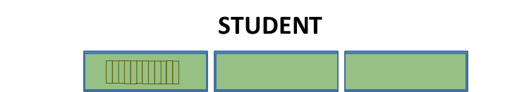
To illustrate the optimization process, consider a query that retrieves the last names and first names of students enrolled in a specific course. Given the following tables:
The SQL query is structured as follows:
SELECT LastName, FirstName
FROM Student, Exam
WHERE Student.ID = Exam.SID AND Exam.CourseID = 'DB2';
This query can be represented through a query tree, where each node corresponds to an operation, such as selecting rows or projecting specific columns. The tree indicates the logical flow of operations, starting from the projection of last names and first names, moving through the selection based on student IDs, and finally filtering exams for the specified course.
graph LR
    A[π LastName, FirstName] --> B[σ Student.ID = Exam.SID] --> C[σ Exam.CourseID = 'DB2'] --> X((x))

    X --> D[Student]
    X --> E[Exam]
The DBMS optimizes the query in several ways, including restructuring the query tree to create an equivalent but more efficient version, utilizing database statistics, and selecting efficient implementations for each operator. For example, consider an alternative optimization where the DBMS first filters Exam entries with the specified CourseID before joining with the Student table. This change reduces the number of rows processed in the join, which can significantly enhance performance.
graph LR
    A[π LastName, FirstName] --> B[σ Student.ID = Exam.SID] --> X((x))

    X --> D[Student]
    X --> C[σ Exam.CourseID = 'DB2'] --> E[Exam]
To assess the effectiveness of various optimization strategies, the DBMS relies on statistics regarding the database. In this case, consider the following statistics:
The university has students.
Each student is enrolled in an average of exams.
Only students are taking the course “DB2.”
With this data, the optimizer evaluates the cost associated with each potential query execution plan. It assesses costs for various operations, such as filtering exams by CourseID and joining the results with the student records. By comparing the costs of different execution plans, the optimizer can select the most efficient one.
In the context of relational database systems, relation profiles serve as essential metadata constructs that describe the quantitative characteristics of database tables. These profiles are not concerned with the actual data content per se, but rather with structural and statistical information that supports efficient query processing and system optimization. The information contained in relation profiles is maintained within the data dictionary, a specialized system catalog that stores metadata about the schema and statistics of the database.
One of the core components of a relation profile is the cardinality of a relation, which refers to the number of tuples (or rows) present in a given table. This metric is critical for query optimization, as it helps the database management system (DBMS) estimate the size of the data that will be processed. The DBMS can retrieve this information efficiently using queries like SELECT COUNT(*) FROM T, which often access precomputed values in the data dictionary rather than scanning the entire table.
Another important aspect of relation profiles concerns the dimensions of attributes, or columns. Each attribute is characterized by a specific data type and size, typically measured in bytes. This dimensional information is vital for memory management, especially in operations such as buffer allocation and data transfer during query execution.
The number of distinct values for each attribute is another statistical indicator maintained by the system.
Definition
For a given attribute in table , the number of unique values it can take is denoted by . This measure reflects the degree of variability or selectivity of the attribute, which in turn influences the effectiveness of selection predicates.
Furthermore, relation profiles include minimum and maximum values for each attribute. These boundary values enable the DBMS to make rapid decisions regarding range-based queries and comparisons involving relational operators such as <, >, <=, and >=. By consulting these stored statistics, the system can often eliminate large portions of the data from consideration early in the query evaluation process, thereby improving performance.
Importantly, relation profiles are not static. To remain effective, they must be periodically refreshed to reflect changes in the underlying data. Maintaining up-to-date statistics is crucial for cost-based query optimization, a strategy in which the DBMS selects execution plans based on estimates of resource consumption. Accurate relation profiles allow the optimizer to make informed decisions about join order, indexing strategies, and access paths, ultimately leading to more efficient query execution.
Data Profiles and Selectivity of Predicates
Data profiles focus on the selectivity of predicates in query conditions.
Definition
Selectivity is defined as the probability that a given row will satisfy a specific predicate.
For an attribute with (indicating that can take on distinct values), and assuming a uniform distribution of values across tuples, the selectivity of a predicate in the form can be expressed as .
Example
For example, if , the selectivity for the predicate City = 'SomeCity' would be , translating to a 0.5% probability of any randomly selected row meeting the condition. Given a population of students and an average of students per city, this estimation suggests that about students would reside in each city on average.
In scenarios where data distribution information is lacking, the DBMS generally assumes a homogeneous distribution of values, which simplifies the estimation process but may lead to inaccuracies in specific cases.
Operations and Access Methods
The efficiency of query execution is also influenced by the choice of operations and access methods.
Operations
Access Methods
Description
Selection
Sequential access
This operation retrieves rows that satisfy a certain predicate. It typically employs sequential access methods, scanning through the dataset to find matching tuples.
Projection
Hash-based indexing
This operation focuses on extracting specific columns from the rows. Hash-based indexing is commonly used to optimize projection, allowing for faster access to relevant attributes.
Sorting
Tree-based indexing
When data needs to be ordered based on specific attributes, tree-based indexing is an effective method. It allows for efficient traversal and retrieval of ordered data.
Joining
Varies
The method of joining tables can vary widely based on the DBMS implementation, with various algorithms (e.g., nested loop, hash join) potentially used to optimize performance.
Grouping
Varies
Similar to joining, the approach to grouping data for aggregation can differ based on the underlying database system, necessitating careful consideration of the method used for optimal performance.
Sequential Scan
A sequential scan is a fundamental method employed by DBMS to access and retrieve data from tables or intermediate results. This process involves sequentially accessing all tuples (rows) within a specified table and simultaneously executing various operations, such as projection and selection.
In the context of a sequential scan, projection refers to the operation of selecting a specific subset of attributes (or columns) from the tuples in a table. This allows the DBMS to retrieve only the necessary information, reducing the amount of data processed and returned to the user. Meanwhile, selection involves applying a simple predicate, typically in the form of , where represents an attribute and signifies a specific value. This process filters the tuples, allowing the DBMS to retrieve only those that meet the specified condition.
Sequential Scan Example
To illustrate the concepts of sequential scans and access methods, let’s consider a practical example involving two tables: STUDENT and EXAM.
STUDENT Table:
Total Tuples:
Each Tuple Size: bytes (calculated as 4 bytes for ID, 25 for Name, 25 for LastName, 25 for Email, 12 for City, 3 for Birthdate, and 1 for Sex)
Block Size: 8KB (8,192 bytes)
Block Factor: tuples per block
Total Blocks: blocks
EXAM Table:
Total Tuples:
Each Tuple Size: bytes (calculated as 4 bytes for SID, 4 for CourseID, 3 for Date, and 4 for Grade)
Block Factor: tuples per block
Total Blocks: blocks
If we execute the query SELECT * FROM STUDENT WHERE City = 'Rome';, the DBMS will perform a sequential scan on the STUDENT table. Given that the City attribute is not indexed, the DBMS must examine each tuple to determine if it meets the condition. This results in a total of I/O accesses to retrieve the relevant tuples from the STUDENT table.
However, if we perform a query like SELECT * FROM STUDENT WHERE ID < 500;, the DBMS can optimize the sequential scan by leveraging the ordering of the data. In this case, it can stop scanning once it reaches the first tuple where ID >= 500, effectively reducing the number of I/O accesses required to retrieve the relevant tuples.
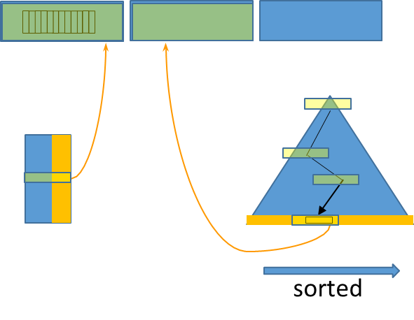
Hashing and Tree-Based Indexing
Hashing is a technique primarily supporting equality predicates. It allows for rapid data retrieval based on exact matches. When a query includes a condition such as , hashing can provide quick access to the desired tuples without scanning the entire dataset.
On the other hand, tree-based indexes offer a broader range of capabilities. They support selection and join criteria, enabling efficient retrieval of related tuples from multiple tables. Furthermore, tree-based indexes are instrumental for operations that involve sorting, such as ORDER BY and GROUP BY clauses, as well as for eliminating duplicates through operations like UNION and DISTINCT.
Predicate-Based Access (Lookup)
Predicate-based access, often referred to as lookup, is an efficient mechanism used by DBMS to retrieve data based on specified conditions or predicates. Indexes built on attributes facilitate rapid access to data for queries that use these attributes as filters. The types of predicates that can leverage indexing include:
Simple Predicates: These are straightforward conditions of the form , where is a specific value.
Interval Predicates: These include conditions that specify a range of values, such as , , or .
The cost associated with lookups varies depending on the underlying data structure utilized for indexing.
The cost of performing lookups is influenced by the storage structure being used:
Sequential Structures:
These structures do not inherently support efficient lookups, resulting in a full table scan for access, which can be costly in terms of performance. However, if the data is stored in a sequentially ordered manner, the cost can be reduced somewhat, as the DBMS may stop searching once the desired condition is met.
Hash and Tree Structures:
Lookups are supported when is designated as the search key attribute of the structure. The lookup cost will depend on several factors:
Storage Type: This includes whether the index is primary or secondary.
Search Key Type: The nature of the keys, whether they are unique or non-unique, plays a significant role in determining lookup costs.
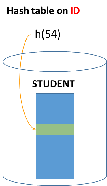
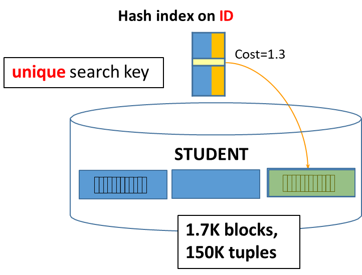
Equality Lookup on a Primary and Secondary Hash
Consider the following SQL query that aims to retrieve a specific student record based on the unique identifier:
SELECT * FROM STUDENT WHERE ID = '54';
In this case, the query predicate directly targets the search key (). Assuming there are no overflow chains, the DBMS can access the block containing the tuple with directly, resulting in a cost of I/O access. However, if there are overflow chains (additional data that might be stored elsewhere due to collisions in the hash structure), the cost may increase. For instance, if the cost of handling overflow chains is , the total cost would be I/O accesses.
Now, consider the same SQL query, but this time using a secondary hash index:
When using a secondary hash index, the situation is similar to that of a primary hash index regarding the initial lookup cost. The cost remains I/O access if there are no overflow chains, and I/O accesses if there are overflow chains. However, with a secondary hash, the DBMS must also access the block that contains the full tuple, which adds to the overall cost. Therefore, the total cost for this operation can be represented as:
Cost with overflow chain: I/O accesses (to access the hash index)
Plus an additional access for the block containing the full tuple.
Query Predicate on a Non-Unique Search Key
Consider a query that retrieves students with a specific , which may not be unique across the dataset:
SELECT * FROM STUDENT WHERE LastName = 'Rossi';
In this case, the query predicate targets a non-unique search key, meaning that multiple tuples can correspond to the same . The cost structure for this operation includes the following components:
Initial Access to the Hash Index: The cost remains I/O access. If overflow chains exist, this cost increases by the size of the overflow chain (e.g., ), leading to a total of I/O accesses.
Accessing Full Tuples in Primary Storage: Since the query could return multiple tuples (for example, all students with the last name “Rossi”), additional I/O accesses are necessary. If we assume in a dataset of tuples, we estimate that each last name appears, on average, twice (). Therefore, for each last name, the DBMS would need to follow pointers to access the corresponding tuples.
The total cost of accessing the relevant data in this scenario can be summarized as:
Cost to access the hash index (with overflow chain): I/O accesses.
Plus the cost to access the full tuples needed for the SELECT * operation: I/O accesses (for the two tuples corresponding to “Rossi”).
Consequently, the TOTAL COST for the entire operation becomes I/O accesses.
NOTE
When retrieving data using a non-unique key, we cannot assume that all “Rossi” tuples are stored in the same block of primary storage. This lack of certainty can further influence the I/O costs associated with the query execution.
Equality Lookup on a Primary and Secondary B+ Tree
When performing a lookup on a primary B+ tree, the efficiency of data retrieval is significantly influenced by whether the query predicates target unique keys or non-unique keys.
For instance, consider the following SQL query aimed at retrieving a specific student record using a unique identifier:
SELECT * FROM STUDENT WHERE ID = 54;
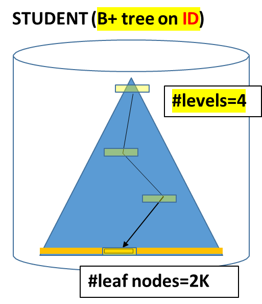
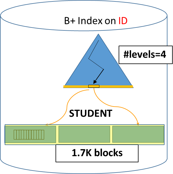
In this case, the search key is unique, meaning that only one tuple corresponds to the key value of . The cost associated with this query involves traversing the B+ tree structure. Specifically, the query requires accessing 3 intermediate levels of the tree and 1 leaf node, resulting in a total of I/O accesses.
It is important to note that the leaf nodes of a primary B+ tree contain the entire tuples, allowing for efficient retrieval once the appropriate leaf node is reached.
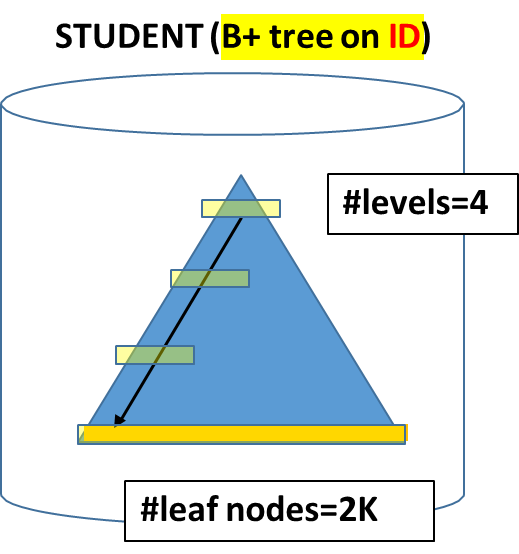
If the query does not use the search key, as in the following SQL statement:
SELECT * FROM STUDENT WHERE City = "Milan";
In this scenario, the DBMS needs to reach and scan all the leaf nodes in the B+ tree to identify relevant records. The cost is considerably higher due to the necessity of scanning through all the leaf nodes. The total cost for this operation would therefore be approximately I/O accesses, combining the 3 intermediate levels accessed and the number of leaf nodes.
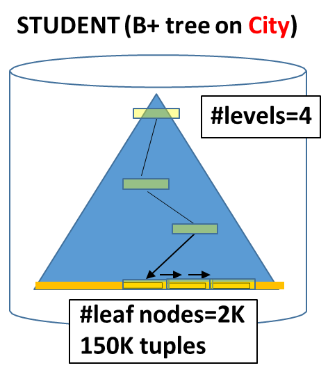
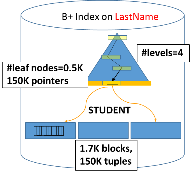
For queries that target a non-unique search key, the access cost calculation involves several factors:
Access Levels: It takes 4 levels to reach the first leaf node.
Statistics: With , we can determine that there are approximately tuples per city, given that the total number of student tuples is .
Leaf Node Capacity: Since each leaf node can contain about tuples ( tuples / leaf nodes), the number of blocks needed for students from “Milan” can be calculated as follows:
Total Milan tuples =
Leaf nodes needed = , which rounds up to leaf nodes.
Combining these, the total cost for the operation amounts to I/O accesses (3 for the intermediate levels and 14 for the leaf nodes).
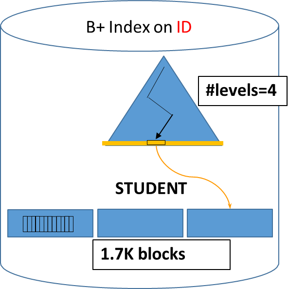
Equality Lookup on a Secondary B+ Tree
Using a secondary B+ tree, consider the following SQL query that retrieves a student record based on a unique identifier:
SELECT * FROM STUDENT WHERE ID = "54";
In this case, the cost for the operation includes accessing 3 intermediate levels of the B+ tree, 1 leaf node, and an additional access for the data block containing the full tuple. Thus, the total cost amounts to I/O accesses.
If the query does not target the search key, as in the example:
SELECT * FROM STUDENT WHERE City = "Milan";
In this case, the index becomes ineffective, and the DBMS would need to perform a full table scan. This full scan incurs a cost of approximately I/O accesses, which is considerably higher than the indexed lookup.
For a query on a non-unique search key, such as:
SELECT * FROM STUDENT WHERE LastName = "Rossi";
We can derive the cost as follows:
Statistics: Assume . Given there are pointers to student tuples, on average, each last name appears approximately twice.
Block Calculation: The number of pointers fitting in each block can be computed:
pointers / distinct last names = pointers per last name.
pointers / blocks = pointers per block, which means 2 tuples fit in one block.
The total cost includes the following components:
Accessing the B+ tree levels: intermediate leaf.
Accessing the blocks containing the student records: blocks.
Thus, the total cost for the query is I/O accesses (3 for intermediate levels, 1 for the leaf node, and 2 for accessing the student records).
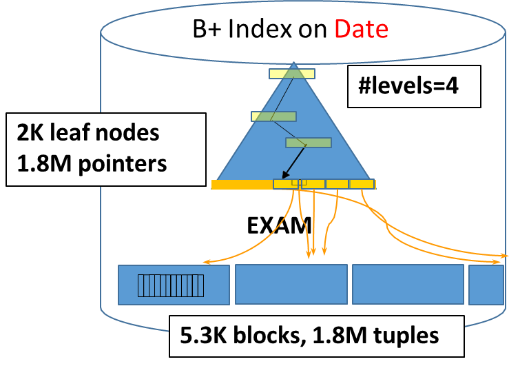
For a query like:
SELECT * FROM EXAM WHERE Date = "10/6/2019";
Assuming , we can compute the number of tuples per date. With a total of million tuples, the average is tuples per date.
The number of leaf nodes that would contain pointers to these tuples can be estimated as follows:
Pointers per leaf node = .
Leaf nodes per date pointers = , which suggests that these pointers would fit across 4 blocks.
Consequently, the cost can be broken down into:
Number of intermediate levels: .
Number of leaf nodes accessed: .
Total number of blocks to access in the EXAM table: (for the pointers to the tuples).
Overall, the total cost for this operation is approximately I/O accesses when accounting for both the intermediate and leaf levels.
It is important to note that the queried date may not be located at the left-most key in the block, necessitating further I/O operations for complete retrieval.
Summary Table: Lookup Costs by Access Method and Key Type
Access Method
Key Type
Cost (I/O Accesses)
Notes
Sequential Scan
Any
Total blocks in table
Full table scan; no index support; cost proportional to table size
Primary Hash
Unique
1 (no overflow), 1.3 (with overflow)
Direct access to block; overflow chains increase cost
Secondary Hash
Unique
2 (no overflow), 2.3 (with overflow)
Index block + data block; overflow chains increase cost
Primary Hash
Non-Unique
1 (no overflow) + pointers
1 for index + 1 per tuple; cost increases with duplicates
Secondary Hash
Non-Unique
1 (no overflow) + pointers
1 for index + 1 per tuple; cost increases with duplicates
Primary B+ Tree
Unique
\#levels (e.g., 4)
Traverse tree to leaf; leaf contains full tuple
Secondary B+ Tree
Unique
\#levels + 1 (e.g., 5)
Traverse tree to leaf + access data block
Primary B+ Tree
Non-Unique
\#levels + \#leaf blocks
Traverse tree; scan all leaf blocks for key; cost depends on duplicates
Secondary B+ Tree
Non-Unique
\#levels + \#leaf blocks + \#tuples
Traverse tree; scan leaf blocks; 1 data block per tuple
Primary B+ Tree
Interval
\#levels + \#leaf blocks in interval
Traverse to first leaf; scan linked leaves for range
Secondary B+ Tree
Interval
\#levels + \#leaf blocks + \#tuples
Traverse to first leaf; scan leaves; 1 data block per tuple in interval
Legend:
#levels: Number of intermediate tree levels traversed (typically 3–4)
#leaf blocks: Number of leaf blocks containing matching keys
#tuples: Number of matching tuples (for non-unique or interval queries)
Overflow: Additional cost due to hash collisions
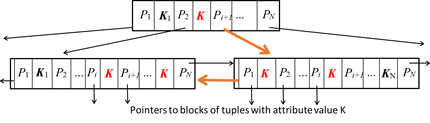
Indexes on Non-Unique Attributes
When a B+ tree index is created on a non-unique attribute, multiple tuples can be associated with the same search key. This results in several pointers within the leaf nodes pointing to the tuples corresponding to that key. Here are some important points to consider:
Multiple Leaf Nodes:
It’s possible for the B+ tree to have multiple leaf nodes corresponding to the same key value. These nodes may contain pointers to tuples with identical values for the indexed attribute. There may also be intermediate nodes that contain keys present in the first position of multiple leaf nodes.
Key Order:
Each level of the B+ tree will maintain a sorted order of keys, where . This ordering applies not only to the leaf nodes but also to the intermediate nodes.
Search Algorithm Modification:
When searching for a key, once a leaf node is reached, if the search key is found as the first key in that node, the algorithm must also check the preceding sibling. This necessitates the use of a doubly linked list among leaf nodes to facilitate traversal. The search continues through the chain of leaf nodes until a key greater than is encountered.
Interval Lookups Ai<v, v1 ≤Ai≤v2
Interval lookups enable the retrieval of data tuples that fall within a specified range of values for a given attribute. This capability is exemplified in SQL queries such as
SELECT * FROM EXAM WHERE Date < "10/6/2019"SELECT * FROM EXAM WHERE Date BETWEEN "10/6/2019" AND "10/10/2019"
The efficiency with which these lookups are performed is heavily dependent on the underlying physical data structures employed by the database.
Sequential and hash-based storage structures inherently lack efficient mechanisms for interval lookups. In both cases, the absence of an ordered arrangement of data based on the lookup attribute necessitates a full table scan, where every record must be examined to identify those that satisfy the interval criteria. This leads to a performance bottleneck, particularly for large datasets.
Conversely, tree-based indexing structures, specifically B+ trees, are well-suited for supporting interval lookups, provided that the indexed attribute serves as the search key.
The performance and cost associated with these lookups are influenced by whether the B+ tree is a primary or secondary index and whether the key values are unique or non-unique.
When an interval lookup, such as , is performed on a primary B+ tree, the process begins by accessing the root node. Subsequently, one node at each intermediate level of the tree is read until the first leaf node containing tuples where is located. From this point, if all the required tuples within the specified range ( to ) reside within the initial leaf block, the search can be terminated. However, if the interval spans beyond this single block, the search continues by traversing through the horizontally linked leaf nodes until all tuples up to have been retrieved. The total cost for such an operation is calculated as the sum of 1 block access for each intermediate level traversed and the number of additional leaf blocks that must be accessed to encompass all tuples within the defined interval.
Similarly, an interval lookup on a secondary B+ tree follows a comparable procedure. The operation initiates with reading the root node, followed by accessing one node at each intermediate level until the first leaf node is reached. This leaf node contains pointers to data records where . If all the necessary pointers to tuples within the range up to are contained within this initial leaf block, the search concludes. Otherwise, the traversal continues through the linked leaf nodes, accessing additional blocks that contain pointers until the threshold is met. The cost associated with this process includes 1 block access for each intermediate level, plus the block accesses required for any additional leaf blocks accessed to retrieve all pointers within the interval. Crucially, an additional data block access is incurred for each pointer retrieved, as this is necessary to fetch the actual data tuple from the data file.
Predicates in Conjunction and Disjunction
Predicates in conjunction and disjunction refer to the logical operations used in SQL queries that combine multiple conditions in the WHERE clause.
SELECT *FROM STUDENTWHERE City = "Milan" AND Birthdate = "12/10/2000"
In this case, both conditions must be true for a tuple to be included in the result. If indexes support the predicates, the Database Management System will choose the most selective predicate (the one that filters the most rows) for data access. The remaining predicates will be evaluated in main memory, which can improve performance by reducing the number of rows that need to be scanned from the disk.
SELECT *FROM STUDENTWHERE City = "Milan" OR Birthdate = "12/10/2000"
For disjunction, at least one of the conditions must be true for a tuple to be included in the result. If all predicates have corresponding indexes, the DBMS can utilize the indexes for each condition, but this may require duplicate elimination to ensure that the same tuple is not included multiple times in the result set. If any of the predicates lack supporting indexes, a full scan of the relevant table must be performed, which can significantly impact performance.
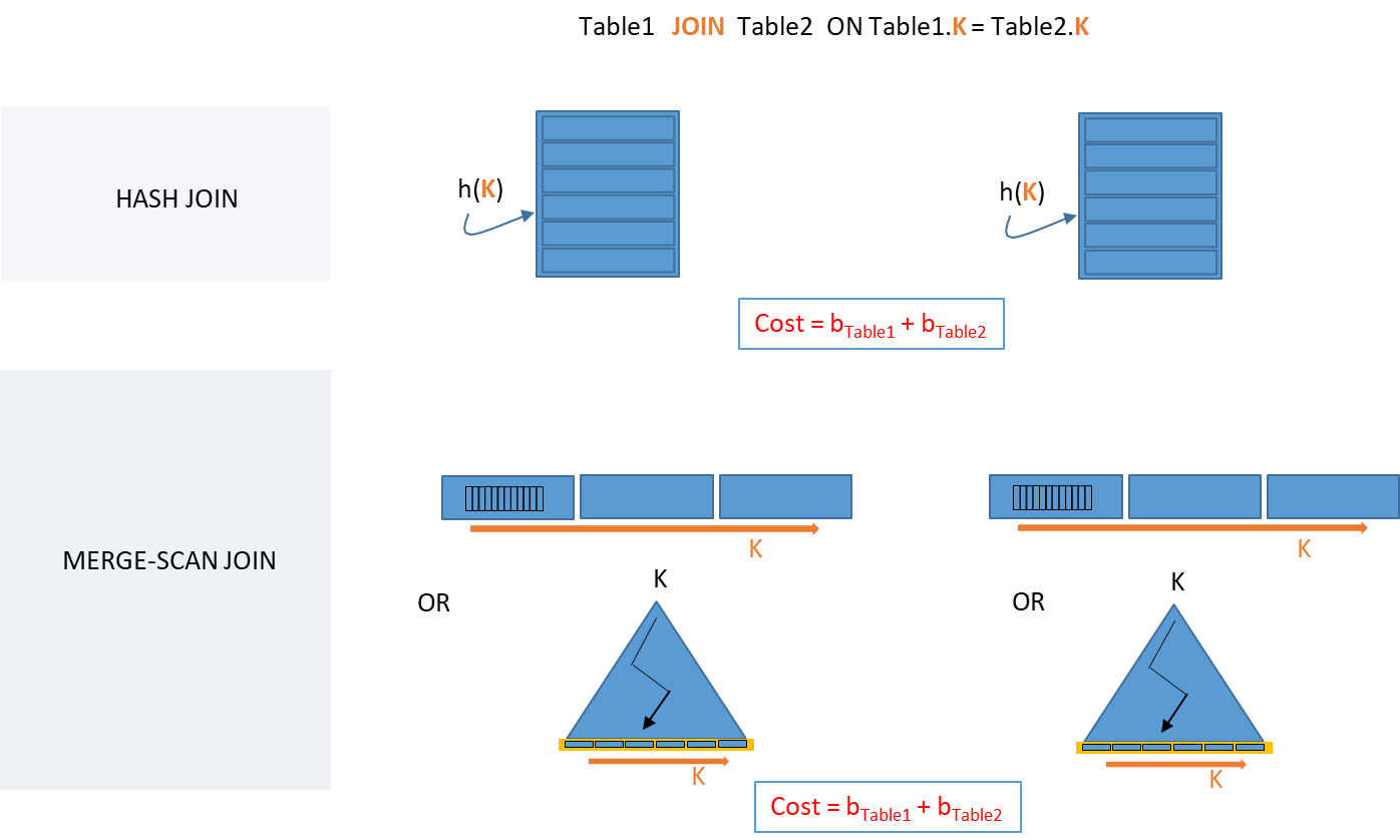
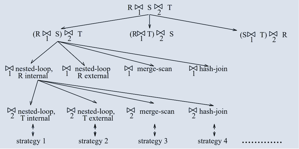
Join Methods
Join operations are fundamental in relational databases, facilitating the combination of rows from multiple tables based on a common field, typically a primary or foreign key. Despite their necessity, joins are often resource-intensive and can impact database performance, especially when dealing with large datasets. Database management systems employ several join strategies, each tailored to different data characteristics and optimized for specific scenarios. The primary join methods include:
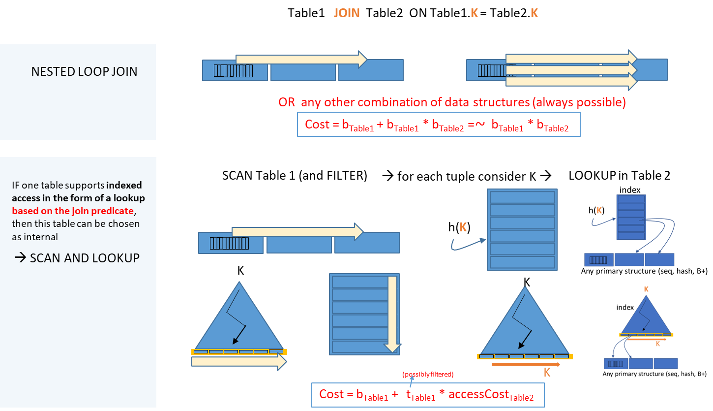
The Nested-Loop Join is the simplest form of join operation, where each row in the first table is compared with every row in the second table to find matching rows based on the join condition. This approach is intuitive but can be computationally expensive for large datasets, as its time complexity is generally , where and are the number of rows in each table. Therefore, nested-loop joins are often more suitable for small tables or scenarios where more efficient indexing is not feasible.
The Merge-Scan Join offers a more efficient alternative when both tables are pre-sorted on the join key. This join strategy sequentially scans each sorted table, merging rows based on the join condition. The merge-scan join is highly efficient for equi-joins (joins where the relationship is based on equality) because it takes advantage of sorted data to avoid repetitive scans. Its time complexity is closer to , making it significantly faster than a nested-loop join for large datasets. However, this method requires that both tables be sorted in advance. This makes merge-scan joins particularly beneficial in data warehousing environments, where data may be loaded in sorted order or periodically sorted for efficient querying.
The Hashed Join is commonly used for equi-joins and works by building a hash table based on the join key for one of the tables, typically the smaller one. The second table is then scanned, and each row is checked against the hash table for matches. This approach leverages the rapid lookup capabilities of hash tables, making it efficient and reducing the need for repeated scanning of rows. The hashed join is particularly advantageous when memory is sufficient to hold the hash table for the smaller dataset, as it minimizes disk I/O. Its time complexity approximates , like the merge-scan join, but with a more random access pattern rather than sequential. Hashed joins are widely used in query optimizations for relational databases, especially in transactional systems and for tables where data is not sorted or indexing is impractical.
Selecting the optimal join method depends on several critical factors, which database administrators and query optimizers take into account to ensure efficient performance.
The size of the tables is a primary consideration, as smaller tables can often benefit from hashed joins, while larger, sorted datasets may align better with merge-scan joins.
The availability of indexes on join keys can also be a determining factor; indexed columns make nested-loop joins more feasible by reducing the number of rows that need to be scanned.
Additionally, the distribution of the data (such as the uniqueness or duplication of values in join columns) influences performance, as highly unique keys can reduce the need for duplicate elimination and make certain join types more efficient.
Memory constraints are another consideration; the availability of sufficient memory for hashing can enable hashed joins, while limited memory might necessitate a nested-loop approach if indexing and sorting are unfeasible.
Finally, the expected size of the output—especially in joins where one table significantly outnumbers the other—can affect whether duplicate elimination or aggregation will add further processing needs.
Example
The STUDENT Table contains a total of records (referred to as “tuples”) with each tuple requiring about 95 bytes of storage. Here is a breakdown of the storage requirements for each field:
ID: 4 bytes
Name: 20 bytes
LastName: 20 bytes
Email: 20 bytes
City: 20 bytes
Birthdate: 10 bytes
Sex: 1 byte
Given a block size of 8 KB (8192 bytes), we calculate the Block Factor to determine how many tuples can fit in one block. By dividing the block size by the tuple size, we find that each block can hold approximately 87 tuples:
Consequently, to store all 150,000 records, the Total Blocks required for the STUDENT table is calculated as follows:
The EXAM Table, on the other hand, contains tuples, each requiring 24 bytes of storage, with the storage breakdown as follows:
SID: 4 bytes
CourseID: 4 bytes
Date: 12 bytes
Grade: 4 bytes
For this table, the Block Factor is calculated similarly, with each block capable of holding approximately 340 tuples:
This means the Total Blocks required for the EXAM table is:
Equality Joins With One Join Column
SELECT * FROM STUDENT JOIN EXAM ON ID = SID
In relational algebra, this join can be represented as:
This equality join links the ID from the STUDENT table with the SID from the EXAM table.
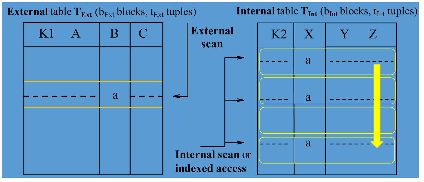
Nested-Loop Join
A nested-loop join is one of the simplest and most intuitive methods for joining two tables in a database. It works by scanning the external table and, for each block of that table, scanning the internal table to find matching tuples.
It compares the tuples of a block of table (the external table) with all tuples of a block of table (the internal table). The process continues until all blocks of the external table have been processed. We always assume that the buffer does not have enough available free pages to host more than a few blocks of the internal table, which is why it is referred to as a “nested-loop” join.
General Cost Calculation: The cost of a nested-loop join is influenced by the number of blocks in both tables:
where, is the number of blocks in the external table, and is the number of blocks in the internal table.
Optimal Scenario: If one of the tables is small enough to fit entirely in memory (buffer), it is chosen as the internal table:
Example
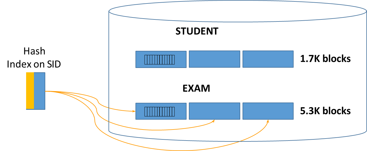
In a simple nested-loop join, each row in one table is compared with every row in another table to identify matching entries based on a join condition. Here, the join operation is performed between two tables, STUDENT and EXAM, based on the ID in STUDENT matching the SID in EXAM. This join type, although straightforward, can be computationally expensive, especially as table sizes increase, due to the high number of I/O operations required.
The STUDENT table occupies approximately blocks (). The EXAM table is larger, occupying around blocks ().
The join operation is represented by the following SQL query:
SELECT STUDENT.* FROM STUDENT JOIN EXAM ON ID = SID
In a nested-loop join, the cost is calculated based on the number of I/O accesses required to perform the join. The cost depends on which table is designated as the “external” (outer) table and which as the “internal” (inner) table, as this affects the number of times each block needs to be read:
When STUDENT is the external table: Each block in STUDENT is read once, and for each block, the entire EXAM table is scanned to find matching rows. This results in a cost of:
When EXAM is the external table: In this case, each block in EXAM is read once, and for each block, the STUDENT table is scanned. This also results in:
Regardless of which table is chosen as the external or internal, the cost remains approximately the same, totaling around 9 million I/O operations. This high number of accesses illustrates why nested-loop joins can be costly for large datasets and why alternative join methods (such as hashed joins or merge-scan joins) may be preferable when table sizes are substantial.
Nested-Loop Joins with Caching
Caching can significantly enhance the efficiency of nested-loop joins by storing the smaller table (the “internal” table) entirely in memory, reducing the need for repetitive disk I/O operations. This method is effective when the internal table is small enough to fit into cache, minimizing the need to read each block multiple times.
Example with Cached CITIES Table
Consider a scenario where a small table, CITIES, is used in a join operation with a larger table, STUDENT.
The CITIES table is small, occupying only 10 blocks, making it suitable for caching (with a block size of 8KB, totaling 80KB). By storing CITIES in memory, each block in STUDENT can be scanned and joined with the cached blocks of CITIES, significantly lowering the total I/O cost.
SELECT STUDENT.* FROM STUDENT NATURAL JOIN CITIES
Cost Calculation:
Cache the CITIES Table: All 10 blocks of CITIES are read into memory once, resulting in just 10 I/O accesses.
Scan the STUDENT Table: With CITIES cached, only the STUDENT table’s blocks need to be scanned, totaling 1.7K I/O accesses.
Total Cost:
Filters on join conditions can further optimize nested-loop joins by reducing the number of rows processed, though the approach varies based on where the filtering occurs. Below are two options for filtering: applying the condition to the STUDENT table or to the EXAM table, each with distinct cost implications.
Filter the External Table First
In this approach, we apply a filter to the STUDENT table to “only include students located in Milan and having received a grade of 30”. This allows us to narrow down the STUDENT table before joining it with EXAM.
SELECT STUDENT.*FROM STUDENT JOIN EXAM ON STUDENT.ID = EXAM.SIDWHERE City = 'Milan' AND Grade = '30'
Scan STUDENT Blocks: All 1.7K blocks in STUDENT must be read initially, totaling I/O accesses.
Filter Students by City: With an average of 150 cities represented in STUDENT, we can estimate the filtered result for Milan to include around:
Join Filtered Students with EXAM: For these students, each one must join with all blocks in the EXAM table, totaling:
Total Cost:
Filter the Internal Table First
In this option, we start by filtering the EXAM table, selecting only the rows with a grade of 30. This initial reduction is beneficial if EXAM contains numerous grades.
Scan EXAM Blocks: First, we read all blocks in EXAM, totaling I/O accesses.
Filter Exams by Grade: Assuming possible grades in EXAM, we can estimate:
Join Filtered Exams with STUDENT: Each of these exams must be joined with all blocks in STUDENT, resulting in:
Total Cost:
Indexed Nested Loop Join
In an indexed nested loop join, one table can be accessed via an index based on the join predicate. This method reduces the number of I/O operations by allowing direct access to matching tuples in the internal table without performing a full scan.
The cost of an indexed nested loop join is significantly lower than that of a standard nested loop join, especially when one table has an index that supports the join condition.
Selection of Internal Table: If one table supports indexed access, it can be chosen as the internal table to exploit this indexing for quicker access to joining tuples. If both tables support lookups on the join predicate, the one with the more selective predicate is selected as internal.
Cost Components: The total cost is calculated as follows:
Here, is the number of blocks in the external table, and is the number of tuples in the external table.
Consider the following query:
SELECT STUDENT.*FROM STUDENT JOIN EXAM ON STUDENT.ID = EXAM.SIDWHERE City = 'Milan' AND Grade = '30'
Tables:
STUDENT: blocks, filtered for City.
EXAM: Indexed by SID, supporting indexed access.
is the number of different cities in the database
Using a secondary hash index on EXAM allows for optimized access.
Cost Breakdown:
Scan STUDENT: I/O accesses.
Filtered Students: students.
Hash Index Access: For each of the students, access the hash index to find matching exams. Assume no overflow chains.
Exam Access: On average, for each student, there are exams to retrieve.
Total Cost:
When the goal is to check the existence of matching tuples rather than retrieving all columns, the cost can be further reduced:
SELECT STUDENT.*FROM STUDENT JOIN EXAM ON STUDENT.ID = EXAM.SIDWHERE City = 'Milan'
Cost Calculation:
Scan STUDENT: I/O accesses.
Filtered Students: Again, results in students.
Hash Index Access: For each student, access the hash index to check existence.
Total lookups required are only access per student.
Total Cost:
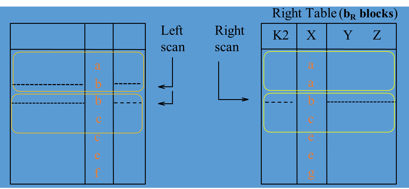
Merge-Scan Join
A merge-scan join is an efficient way to join two tables that are already sorted on the join attribute. This method requires both tables to be ordered according to the same key attribute, which is also used in the join predicate.
Steps
Prerequisite: Both tables must be sorted on the join key.
Execution:
Scan both tables simultaneously.
Compare the current values of both tables:
Advance in the table with the lesser value.
If values match, output the tuple pair <l, r>.
Output: The result will include all combinations of matching tuples from the two tables.
The cost is linear in the size of the tables:
where and are the number of blocks in the left and right tables, respectively.
If a table needs to be sorted, we need to also add the cost of the sorting operation:
Ordered Full Scan: This is possible if the primary storage is sequentially ordered with respect to the join attribute or if a B+ tree index on the join attribute is defined.
Sorting Cost: If tables need to be sorted prior to the merge, add the cost for sorting:
where the number of passes can be calculated as: with being the number of blocks and being the number of buffer pages.
Example: Merge-Scan Join on Ordered Tables
SELECT STUDENT.* FROM STUDENT JOIN EXAM ON ID = SID
Case 1: Both Tables Sequentially Ordered
STUDENT: Sequentially ordered by ID.
EXAM: Sequentially ordered by SID.
Cost:
Case 2: STUDENT Ordered, EXAM with Primary B+ Index
STUDENT: Sequentially ordered by ID.
EXAM: Primary storage with a B+ tree on SID.
Cost:
Assuming 3 intermediate nodes and leaf nodes:
Case 3: STUDENT Ordered, EXAM with Secondary B+ Index
STUDENT: Sequentially ordered by ID.
EXAM: Secondary index on SID.
Cost:
Assuming 3 intermediate nodes and leaf nodes:
Indexed Merge Scan Join
When additional filtering is applied, such as selecting specific grades, the cost can significantly increase.
SELECT S.SIDFROM STUDENT S JOIN EXAM E ON ID = SIDWHERE GRADE > 17
STUDENT: Sequentially ordered by ID.
EXAM: Secondary index on SID.
Cost: The cost of accessing both the intermediate nodes and leaf nodes, plus the number of tuples in EXAM:
Assuming:
intermediate nodes
leaf nodes
tuples in EXAM
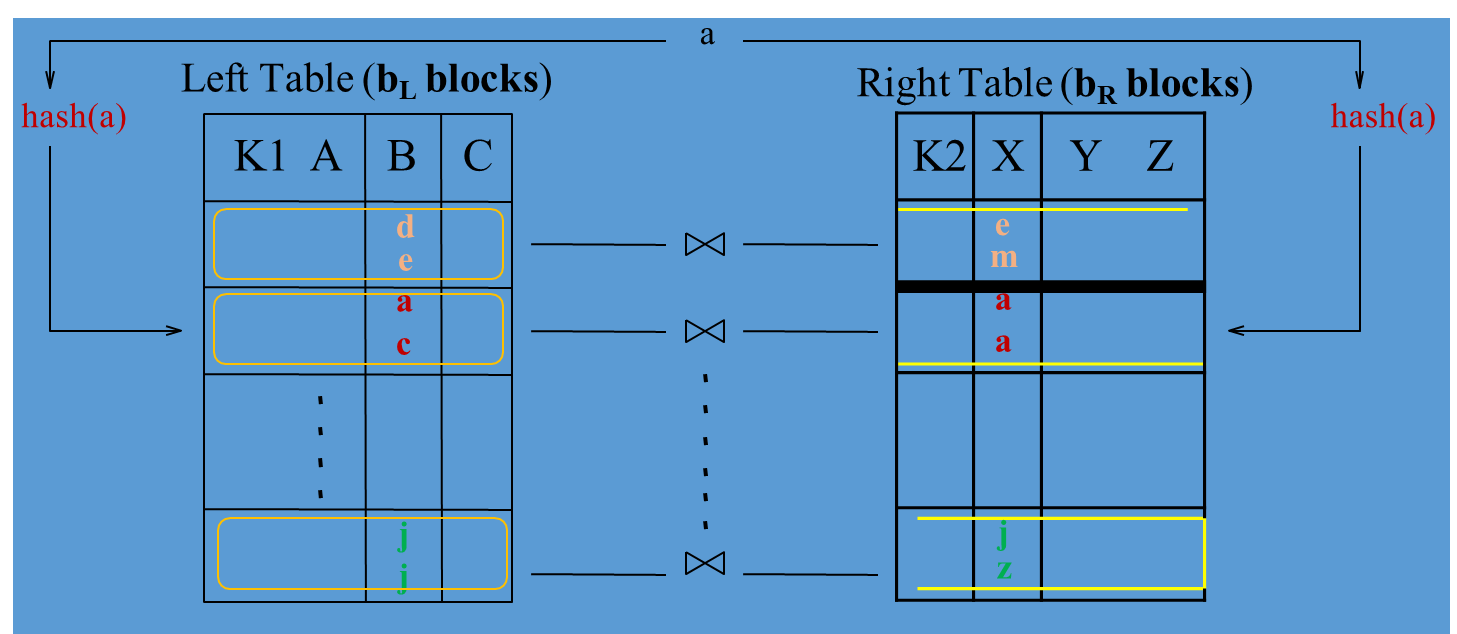
Hashed Join
A hashed join is an efficient method for joining two tables based on a common attribute, particularly when both tables are hashed on the join key. This method can significantly reduce the search space for matching tuples, as they can only be found in corresponding buckets.
Steps
Hashing: Both tables are hashed on the join attribute, which creates a number of buckets. Each bucket will contain tuples that hash to the same value for the join attribute.
Bucket Matching: During the join operation, only the buckets with matching hash values are examined, allowing for quick identification of matching tuples.
Output: The result consists of the combinations of matching tuples from both tables.
The cost of a hashed join is linear with respect to the number of blocks in the hash-based structure. If both tables are primary storage (i.e., the hashed structure is stored as part of the primary storage), the cost can be calculated as:
where:
= number of blocks in the left table.
= number of blocks in the right table.
NOTE
Buckets: While both hashed tables will have the same number of buckets, the actual number of blocks ( and ) may differ slightly due to overflow handling. Overflows occur when multiple tuples hash to the same bucket and the bucket becomes full.
Efficiency: The hashed join is particularly efficient for large datasets when the hash function evenly distributes tuples across the buckets, minimizing the number of comparisons needed.
Example of Hashed Join
Consider the following SQL query that joins the STUDENT table and the EXAM table on the condition where ID from STUDENT matches SID from EXAM:
SELECT S.* FROM STUDENT S JOIN EXAM E ON S.ID = E.SID
To analyze the cost of this hashed join, we need to consider the number of blocks for each table:
The STUDENT table consists of approximately blocks ().
The EXAM table consists of about blocks ().
The steps for the hashed join are as follows:
Building the Hash Table: First, the hash table is created for the smaller table, which in this case is the STUDENT table. This requires reading all blocks of STUDENT into memory.
Probing the Hash Table: Next, each block of the EXAM table is scanned to find matching entries in the hash table. This requires reading all blocks of EXAM.
The total cost of the hashed join can thus be calculated as:
The hashed join method is notably more efficient than nested-loop joins, especially when dealing with large datasets. In this scenario, the total I/O cost of is significantly lower than what would be encountered with a nested-loop join, demonstrating the effectiveness of hashing for reducing the number of required I/O operations during the join process.
Sorting in Databases
Sorting is essential in databases for organizing and quickly retrieving data based on specific attributes. Efficient sorting algorithms can improve query performance, index maintenance, and data processing in relational database systems. There are two primary methods for sorting, depending on the size of the data:
In-Memory Sorting: For data that fits into main memory, algorithms like quicksort and merge sort are typically used. These algorithms offer fast sorting for smaller datasets, allowing the entire data to be processed in-memory without repeated disk access.
External Sorting: For larger datasets that cannot fit into memory, external sorting becomes necessary. This approach involves reading, sorting, and merging blocks of data in chunks that fit into memory. The most common method for this type is external merge sort, which efficiently handles large files by sorting manageable chunks and then merging them into a fully sorted sequence.
External Merge Sort
External merge sort is structured to handle files that exceed memory capacity by processing and merging data in multiple passes. Each pass involves reading data into memory in blocks, sorting it, and writing it back in a way that each subsequent pass combines larger and larger sorted sequences until the entire dataset is sorted.
Algorithm
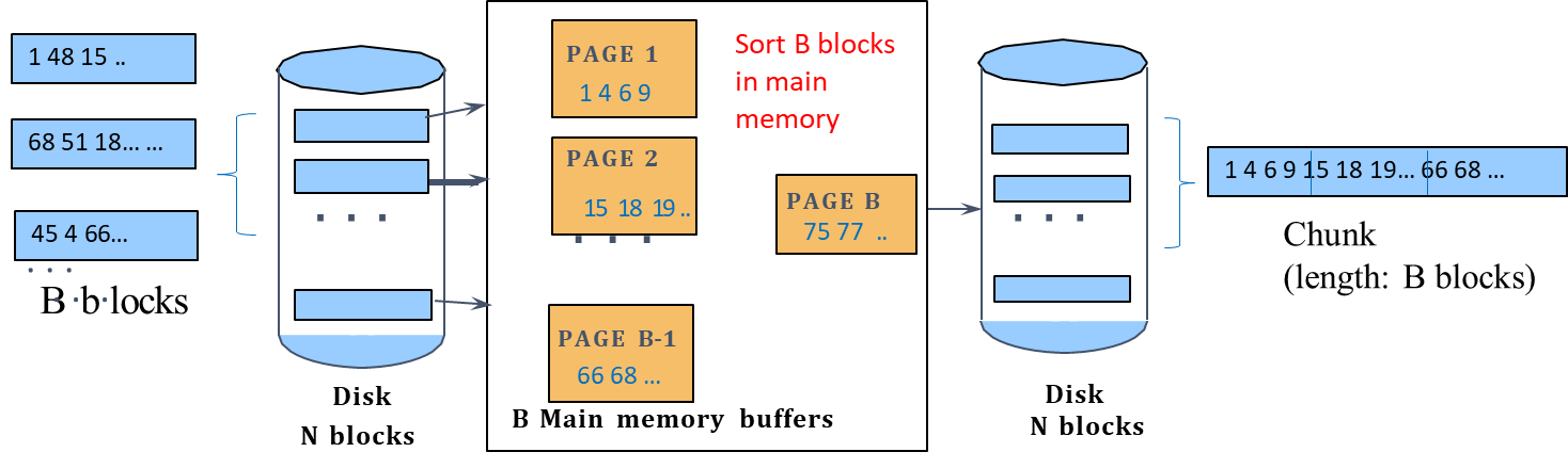
Initial Pass:
In this pass, blocks of data are read into memory, sorted, and then written to temporary files, often called chunk files. This initial sorting creates smaller sorted chunks, each representing a portion of the data.
Calculation of Chunks: If represents the total number of blocks and is the number of blocks that fit into memory, the number of sorted chunks created can be calculated as:
Cost for Initial Pass: This pass requires reading and writing each block once, resulting in a cost of I/O operations (one read and one write per block).
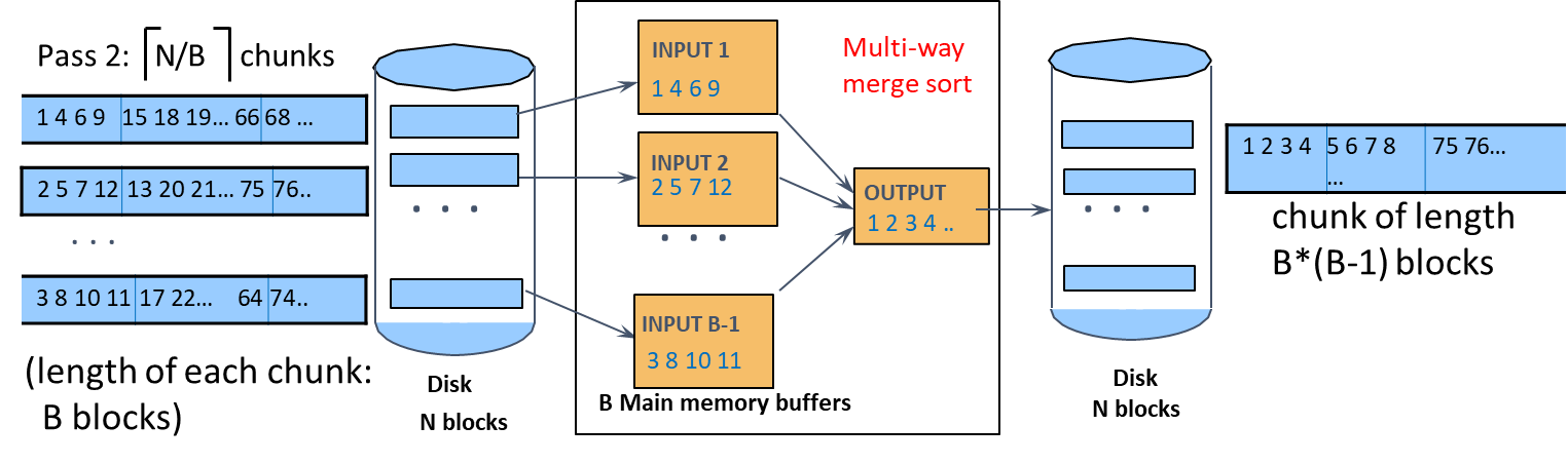
**Subsequent Passes:
In each subsequent pass, the algorithm uses B-1 blocks for reading sorted chunks and one block for writing the merged output.
During each pass, the smallest record among the sorted chunks is selected and written to the output. Once the output buffer is full, it is written to disk.
This process continues until all chunks have been merged into a single, fully sorted file.
Example of External Merge Sort
Suppose we have N = 40 blocks to sort and can only fit B = 5 blocks into memory at a time.
Initial Pass:
We read blocks at a time, sort them, and write each sorted chunk to disk.
Total I/O cost: reads + writes.
Outcome: sorted chunks, each containing pages.
Subsequent Passes:
Pass 2: We load chunks (using blocks) into memory, merge them, and produce a new chunk of pages.
Pass 3: The final pass merges two -page chunks into a single sorted chunk of pages.
Total Passes:
The total cost of external merge sort depends on the number of passes required. For a given dataset of blocks and a memory buffer size of , the number of passes can be calculated as:
The total cost in terms of I/O operations is then:
This table shows the number of passes required to sort datasets of varying sizes () with different memory buffer sizes ():
N
B=3
B=5
B=9
B=17
B=129
B=257
100
7
4
3
2
1
1
1,000
10
5
4
3
2
2
10,000
13
7
5
4
2
2
100,000
17
9
6
5
3
3
1,000,000
20
10
7
5
3
3
10,000,000
23
12
8
6
4
3
100,000,000
26
14
9
7
4
4
1,000,000,000
30
15
10
8
5
4
Cost-Based Optimization in Databases
Cost-based optimization is a critical aspect of database query processing that focuses on determining the most efficient way to execute a query. This involves analyzing various execution plans and selecting the one with the lowest estimated cost.
Decision Variables:
Data Access Operations: Deciding whether to use a full table scan or index access.
Order of Operations: Determining the sequence in which operations are performed, such as the order of joins.
Method Selection for Operations: Choosing the best join method (e.g., nested-loop, hash join).
Parallelism and Pipelining: Leveraging parallel execution and pipelining to enhance performance.
Optimization Approach:
Cost Estimation: Using profiles and approximate cost formulas to assess the cost of different execution strategies.
Decision Trees: Constructing a decision tree where:
Each node represents a choice in the query execution.
Each leaf node corresponds to a specific execution plan.
Cost Calculation: The total cost of a query plan can be represented as:
Here, represents the cost of I/O operations, represents the CPU cost per operation, and is the number of CPU operations involved.
Plan Selection: Optimizers utilize operations research techniques, such as branch and bound, to efficiently explore the decision tree and identify the plan with the lowest estimated cost. The goal is to obtain a “good” execution plan quickly.
Query Execution
Query execution is the process of executing a SQL query against a database to retrieve or manipulate data. The execution process can vary based on the database management system (DBMS) and the specific query being executed. Here are two common approaches to query execution:
Compile and Store: In this approach, the query is compiled once and stored for subsequent executions (known as a prepared statement). The DBMS retains the compiled internal code and tracks dependencies on specific catalog versions used during compilation. If relevant changes occur in the catalog, the compilation is invalidated, and the query must be recompiled.
Compile and Go: This method involves immediate execution of the query without storing the compiled code. Although not stored, the code may remain in memory temporarily and be available for other executions during that period.
Prepared Statements (MySQL)
Prepared statements are a feature in many relational database management systems (RDBMS) that allow for the pre-compilation of SQL queries. This approach enhances performance and security by separating query structure from data, enabling the reuse of execution plans and preventing SQL injection attacks.
Performance: Prepared statements can be executed multiple times with different parameters without the need for re-parsing and re-compiling the SQL statement, leading to faster execution.
Security: By using placeholders for parameters, prepared statements help prevent SQL injection attacks, as user input is treated as data rather than executable code.
Prepared statements are typically used in applications where the same query is executed multiple times with different parameters, such as in web applications or data processing tasks.
PREPARE my_query1 FROM 'SELECT * FROM users WHERE id = ?';
The query is prepared with a placeholder (?) for the parameter. When executing the prepared statement, the actual value is bound to the placeholder:
EXECUTE my_query1 USING 54;EXECUTE my_query1 USING 2;
During query execution, one of the most critical aspects of performance optimization involves the buffer pool, which acts as a memory-resident cache for database pages.
Definition
A page is the fundamental unit of data storage and transfer between disk and memory, typically containing a fixed-size block of data such as table rows, index nodes, or even compiled execution plans, depending on the DBMS architecture.
When a query is issued, the DBMS attempts to retrieve the necessary pages from the buffer pool before resorting to disk access. If a requested page is already present in the buffer pool, this results in what is known as a cache hit. Cache hits significantly improve performance by eliminating the need to perform time-consuming disk I/O operations. On the other hand, if the requested page is not in memory, a cache miss occurs, forcing the system to read the page from disk and load it into the buffer pool, which is considerably slower.
The types of data stored in the buffer pool are diverse. Primarily, it contains data pages that hold the actual tuples (rows) of database tables. In addition to data pages, the buffer pool often includes index pages, which facilitate efficient data retrieval by allowing the DBMS to quickly locate rows based on indexed attributes. Some database systems also store compiled execution plans in the buffer pool, enabling the reuse of previously optimized query strategies without re-parsing and re-optimizing the same statements.
Since the buffer pool operates within a limited memory space, it cannot accommodate all pages indefinitely. As a result, the DBMS must implement a page replacement policy to determine which pages should be evicted when new pages need to be loaded. A common strategy employed is the Least Recently Used (LRU) algorithm or one of its variants. This policy assumes that pages that have not been accessed recently are less likely to be accessed again in the near future. Thus, when the buffer pool reaches its capacity, the DBMS discards the pages that have remained unused for the longest time, freeing space for new, potentially more relevant data.
We can also deallocate the prepared statement when it is no longer needed: