MOLAP, which stands for Multidimensional Online Analytical Processing, is a classic method for OLAP (Online Analytical Processing) analysis. In MOLAP, data is organized and stored in a multidimensional cube structure, rather than in the typical relational database format. The data is often stored in specialized proprietary formats optimized for multidimensional analysis, which contrasts with the row and column-based structure of relational databases. This method is designed to allow users to quickly retrieve and analyze large amounts of data across various dimensions, making it particularly well-suited for complex analytical queries that involve slicing and dicing data along different axes.
One of the primary advantages of MOLAP is its exceptional performance. The multidimensional cube is built with pre-aggregated data, meaning that complex queries can be executed very quickly. Since the cube structure supports the pre-computation of summary statistics and calculations at the time of its creation, users benefit from highly efficient data retrieval. Operations such as calculating totals, averages, or percentages across multiple dimensions are carried out with minimal delay, making MOLAP ideal for scenarios requiring rapid, interactive analysis of large datasets.
Furthermore, MOLAP systems excel at handling complex calculations. Since calculations are performed during the cube’s creation, these systems are not only capable of processing sophisticated formulas and mathematical operations but can do so with speed. Users do not need to perform calculations on-the-fly during their analysis, which further enhances performance by eliminating the need for real-time computation as queries are processed.
However, there are several limitations associated with MOLAP. One significant drawback is the amount of data that MOLAP can effectively handle. Since all calculations are pre-computed during the cube-building process, MOLAP systems are constrained by the cube’s size. This means that while the underlying data may be vast, the MOLAP cube typically stores only summary-level or aggregated information. The cube’s storage capacity limits the granularity of data it can contain, which can be a problem if detailed, raw data is needed for analysis. If more detailed data needs to be included, the cube may become too large to manage effectively, or the organization may need to create multiple cubes.
Another challenge is the additional investment required for adopting MOLAP technology. MOLAP systems often rely on proprietary software and hardware that may not be available within an organization. Therefore, implementing MOLAP may require significant capital investment to procure the necessary technology, along with the human resources required to manage and maintain the system. This investment is often seen as an obstacle for organizations that do not already have MOLAP infrastructure in place or the expertise to handle the specialized tools.
ROLAP
ROLAP, or Relational OLAP, is an OLAP technology that relies on relational databases to manage and analyze multidimensional data. Unlike MOLAP, which stores data in a multidimensional cube, ROLAP works directly with relational database systems. In this approach, operations typically associated with OLAP, such as slicing and dicing data, are implemented by translating them into SQL queries. Essentially, each action a user performs (e.g., filtering, grouping, or summarizing data) is transformed into a WHERE clause or a series of SQL queries that interact with the underlying relational database tables.
One of the key advantages of ROLAP is its ability to handle large amounts of data. Since it operates on relational databases, which are designed to scale and store vast quantities of data, ROLAP does not face the same limitations on data volume as MOLAP systems. The technology benefits from the relational database’s inherent capabilities, such as indexing and optimization, enabling it to manage large datasets more effectively. Furthermore, ROLAP can leverage the complex functionalities provided by relational databases, such as advanced filtering, joining, and aggregating techniques, which allow for flexible data manipulation.
However, ROLAP also comes with certain limitations. Performance can be a significant issue, especially when working with large datasets. Because each interaction with the data involves executing one or more SQL queries, the system’s response time can be slow, particularly when the data size is large or complex queries are involved. Unlike MOLAP, where data is pre-aggregated and calculations are performed in advance, ROLAP systems need to execute the SQL queries in real-time, which can lead to delays.
Another disadvantage of ROLAP is that it is limited by the functionalities of SQL. Although SQL is a powerful language for querying relational databases, it is not inherently designed to handle complex calculations or multidimensional analysis in the way MOLAP systems can. While ROLAP vendors have worked to address these limitations by integrating advanced functions and allowing users to define custom calculations, SQL remains constrained in its ability to perform sophisticated analysis or calculations beyond its core capabilities. This can be an issue for users needing highly specialized data manipulations or analysis.
A more recent development in OLAP technology is HOLAP (Hybrid OLAP), which combines the benefits of both MOLAP and ROLAP. HOLAP systems aim to take advantage of the high performance of MOLAP for summary-level data while leveraging ROLAP for detailed, transactional-level data. When users need to access detailed information, HOLAP can “drill through” the MOLAP cube to access the underlying relational database, providing detailed insights without sacrificing performance for summary-level queries. By using MOLAP for fast access to aggregated data and ROLAP for handling large volumes of detailed data, HOLAP offers a balanced solution that addresses the strengths and weaknesses of both technologies.
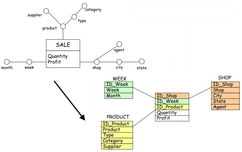
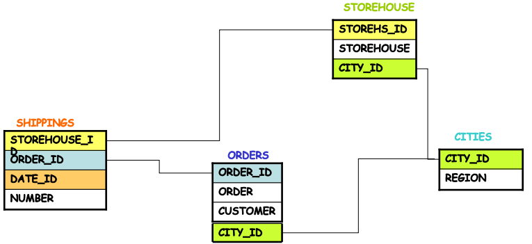
Data Warehouse Logical Design in ROLAP: Star Schema
In the context of ROLAP (Relational OLAP), star schema plays a crucial role in structuring the data for multidimensional analysis. It organizes the data in a way that facilitates efficient querying and reporting, particularly for large-scale data warehouse systems. The star schema consists of a central fact table surrounded by a set of dimension tables. These tables are structured to support high-performance queries and data analysis.
The star schema is built on two key components:
Dimension Tables: A set of relations (e.g., ) represents different dimensions of the data. These dimension tables correspond to various attributes or aspects of the analysis, such as time, product, or location. Each dimension table is characterized by:
A primary key, which uniquely identifies records in the dimension table.
A set of attributes that describe the characteristics of the dimension, such as the product name, store location, or date. These attributes often have varying levels of aggregation.
Fact Table: The fact table, denoted as , contains quantitative data that is being analyzed. It typically includes:
The primary keys from the dimension tables (), which link the fact table to the relevant dimension tables.
Measures or facts, such as sales, profit, quantity, etc. These are the numerical values subject to analysis and aggregation.
The primary key of the fact table is typically a composite key made up of the foreign keys from the dimension tables (i.e., ), ensuring that each row in the fact table is uniquely identified based on the combination of dimension keys. The fact table stores transactional data or aggregate data at different levels of granularity.
Example
For example, consider the Sales data model with the following:
Sales Fact Table (FT): The table records transactional data about sales.
It aggregates sales data across different stores, products, and time periods.
Shop Dimension Table (): This table describes different shops.
Columns: Shop_key, Shop, City, Region.
Shop_key
Date_key
Prod_key
Qty
Profit
1
1
1
170
85
2
1
1
300
150
3
1
1
1700
850
Shop_key
Shop
City
Region
1
COOP1
Bologna
E.R.
2
-
Roma
Lazio
3
-
-
Lazio
In this example, the Sales Fact Table records individual transaction data and aggregate values (e.g., sales for the city of Roma or Lazio). The Shop Dimension Table provides details about each shop, such as its name, city, and region. The key thing to note is that the fact table can include rows that represent aggregated values for higher levels, such as cities or regions, in addition to the individual transaction-level details.
Dimension tables in a star schema are typically denormalized. This means that, for efficiency, attributes may be duplicated to reduce the number of joins required during queries. For example, instead of having separate tables for Product Type and Product Category, these may be included directly in the Product dimension table to simplify queries.
Additionally, surrogate keys are often used in dimension tables. A surrogate key is a system-generated unique identifier used to represent entities in the dimension table. This allows for more efficient storage and quicker lookups compared to using natural keys (e.g., product name or category). The use of surrogate keys ensures better space efficiency and optimizes query performance.
OLAP Queries on Star Schema
Once the data is structured in a star schema, OLAP tools can run complex queries to slice and dice the data, which allows analysts to explore the data across different dimensions. An example of an OLAP query on the star schema is as follows:
SELECT City, Week, Type, SUM(Quantity)FROM Week, Shop, Product, SaleWHERE Week.ID_Week = Sale.ID_Week AND Shop.ID_Shop = Sale.ID_Shop AND Product.ID_Product = Sale.ID_Product AND Product.Category = 'FoodStuff'GROUP BY City, Week, Type;
This SQL query performs the following tasks:
Filters the data based on a specific category ('FoodStuff') in the Product dimension.
Joins the dimension tables (Shop, Product, Week) with the fact table (Sale) to retrieve the relevant data.
Groups the results by City, Week, and Type, providing an aggregated sum of the Quantity for each combination of these dimensions.
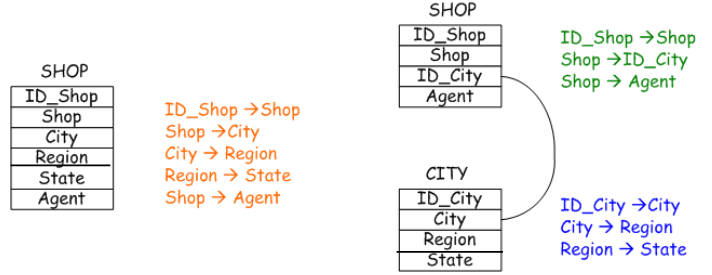
Snowflake Schema
The snowflake schema is an extension of the star schema that aims to address some of the inefficiencies introduced by excessive denormalization in the dimensional tables. While the star schema uses a highly denormalized structure for dimension tables, the snowflake schema normalizes these tables to reduce redundancy and improve data consistency.
The goal of the snowflake schema is to minimize the amount of data duplication by organizing the dimension tables in a way that removes some of the transitive dependencies that occur in the star schema.
In the snowflake schema, the dimension tables are structured in a more normalized form compared to the star schema. Here’s how it works:
Primary Dimension Tables: These are the main dimension tables that correspond to key attributes of the dataset, such as Product, Shop, or Time. These tables contain the primary key for each dimension.
Each dimension table in the snowflake schema consists of:
A primary key , which uniquely identifies records in that dimension table.
A subset of attributes that directly depend on the primary key.
Zero or more foreign keys that allow for the establishment of relationships with other dimension tables.
Secondary Dimension Tables: These tables represent additional levels of hierarchy within the dimensions. For example, the Product dimension may have separate tables for Type and Category, where Category is a higher-level attribute than Type. The foreign keys in the secondary tables point to the primary tables in the schema.
In a snowflake schema, the fact table still contains the foreign keys from the primary dimension tables, but the secondary dimension tables are linked through additional keys. The snowflake schema reduces the redundancy seen in the star schema by storing hierarchical relationships in separate tables.
Example of Snowflake Schema
Consider a scenario with a sales dataset. In the star schema, a Product dimension might include attributes for Category, Type, and ProductName. However, in the snowflake schema, these attributes are placed in separate tables:
Product Dimension: This could contain attributes like ProductID and ProductName.
Product Type Dimension: This contains the TypeID and TypeName, which is linked to the Product table.
Product Category Dimension: This contains CategoryID and CategoryName, linked to the Product Type table.
Similarly, for the Shop Dimension, attributes like City and Region could be separated into different tables to reduce redundancy.
Considerations in the Snowflake Schema
Reduction of Memory Space: By normalizing the dimension tables and removing transitive dependencies, the snowflake schema reduces the amount of data stored. This can lead to more efficient storage, particularly in large-scale data warehouses where reducing redundancy is crucial.
New Surrogate Keys: Like the star schema, the snowflake schema uses surrogate keys—system-generated identifiers for the dimension tables. This ensures more efficient storage and indexing, avoiding the overhead of using natural keys that could be longer or more complex.
Query Performance: The normalization in the snowflake schema can improve performance for queries related to attributes stored in the fact and primary dimension tables. However, queries that involve secondary dimension tables may require more joins, which can slow down performance when compared to the star schema.
Normalization & Snowflake Schema
In the snowflake schema, the normalization process ensures that attributes with transitive dependencies (i.e., attributes that depend on other attributes indirectly) are moved to separate tables. This normalization step results in a structure where data is organized to eliminate redundancy and ensure data consistency.
For example, if there is a transitive dependency between Product Type and Product Category, these attributes would be placed in separate tables to break the dependency chain. As a result, the snowflake schema generally involves more tables than the star schema, but these tables contain less redundant data.
OLAP Queries on Snowflake Schema
When querying a snowflake schema, OLAP tools must join multiple tables, especially for attributes that are stored in secondary dimension tables. Here’s an example of an OLAP query that would work on a snowflake schema:
SELECT City, Week, Type, SUM(Quantity)FROM Week, Shop, Type, City, Product, SaleWHERE Week.ID_Week = Sale.ID_Week AND Shop.ID_Shop = Sale.ID_Shop AND Shop.ID_City = City.ID_City AND Product.ID_Product = Sale.ID_Product AND Product.ID_Type = Type.ID_Type AND Product.Category = 'FoodStuff'GROUP BY City, Week, Type;
In this query:
The Sale fact table is joined with the Product dimension table, which in turn is linked to the Product Type and Product Category tables.
The Shop dimension table is linked to the City table.
The query aggregates data based on multiple dimensions such as City, Week, and Type, and filters data for a specific category ('FoodStuff').
While the query is more complex than one based on the star schema, it is more efficient in terms of storage, as it avoids redundant data by storing hierarchical relationships in separate tables.
Advantages and Disadvantages of Snowflake Schema
Advantages
Disadvantages
Reduced Data Redundancy: By normalizing the dimension tables, the snowflake schema reduces storage space and ensures data consistency.
Complex Queries: The additional joins between tables can make queries more complex and slower compared to the star schema.
Improved Data Integrity: With data distributed across different tables based on hierarchical relationships, updates are easier and less prone to inconsistencies.
Increased Join Operations: While the snowflake schema reduces redundancy, it requires more joins between tables, which can negatively impact query performance, especially for large datasets.
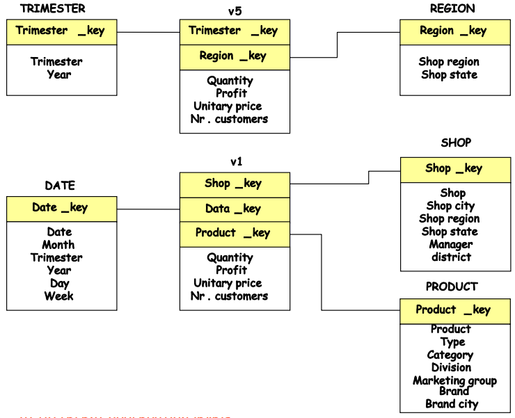
Materialized Views
Materialized views play a critical role in improving performance in OLAP systems by precomputing expensive aggregations and storing them for faster query processing. Unlike regular views, which compute data dynamically during each query execution, materialized views store the result of a query, thus avoiding the need for repetitive computation.
In an OLAP context, aggregation refers to the process of summarizing or condensing large volumes of detailed data into more manageable and meaningful summaries. For example, sales data might be aggregated by product, store, or time period. While aggregation is crucial for providing concise, summarized information, it can be computationally expensive. To mitigate the cost of performing aggregations repeatedly, materialized views store aggregated data at various levels of granularity, making it easy to retrieve precomputed results.
A materialized view can be defined by its aggregation level, which refers to the level of detail or granularity of the data being aggregated:
Primary Views: These represent the most detailed aggregation levels, usually corresponding to the original fact table or a combination of primary dimensions. These views contain detailed data for each fact, such as individual sales transactions.
Secondary Views: These views summarize data at higher aggregation levels, such as by week, month, or region. Secondary views aggregate data from primary views or other secondary views.
The hierarchy of views can be represented as a directed graph, where each view depends on the aggregation of another view. A primary view might serve as the basis for multiple secondary views, each with progressively higher levels of aggregation. For example, if v1 represents the aggregation of sales by product, date, and shop, then v2 could represent sales by type, date, and city, using data from v1.
Here, we see that v2 is an aggregation of v1 at a more general level, v3 is built from v2, and so on. This hierarchy illustrates how materialized views depend on each other based on the level of aggregation.
Partial Aggregations
Sometimes, it’s necessary to introduce derived measures to correctly manage aggregations. Derived measures are calculated by applying mathematical operators to the values in the fact table or another aggregated view. For example, if you have data about sales transactions (product, quantity, price), you might need to compute the profit by multiplying quantity by price. In a materialized view, it’s beneficial to precompute these derived measures to save time during query execution.
Example
Consider the following example:
Type
Product
Quantity
Price
Profit
T1
P1
5
1.00
5.00
T1
P2
7
1.50
10.50
T2
P3
9
0.80
7.20
22.70
Where the Profit is calculated as Quantity * Price. To aggregate this data correctly, you would need to sum the Quantity and Price for each Type and then compute the total Profit.
Type
Quantity
Price
Profit
T1
12
1.25
15.00
T2
9
0.80
7.20
22.70
In this case, the aggregation combines the Quantity and Price for each Type and computes the total Profit. The Profit column is now a derived measure that aggregates across individual transactions.
When working with aggregation, it is important to understand the types of aggregate operators that can be applied:
Distributive Operators: These operators can aggregate data starting from partially aggregated results. Examples include SUM, MAX, and MIN. These operators are relatively simple because they allow data to be combined in any order, making them highly efficient for parallel processing.
Algebraic Operators: These require some additional information to aggregate data correctly. The average (AVG) is an example of an algebraic operator, as it requires the total sum and the count of values to compute the result.
Holistic Operators: These operators are more complex and cannot be derived from partial aggregations. Examples include MODE (most frequent value) and MEDIAN (middle value in a sorted list). These are harder to compute efficiently as they require a full scan of the data.
Relational Schema and Aggregate Data
In a data warehouse, it’s important to manage aggregate data in a way that optimizes performance. Several approaches can be used:
Storing Aggregated Data in the Same Fact Table: In this approach, primary and secondary views are stored within the same fact table. However, for more granular aggregations, the fact table contains NULL values for attributes at finer aggregation levels. This solution is straightforward but might not be the most efficient as data grows.
Using Separate Fact Tables (Constellation Schema): A more optimized solution is to store aggregated data in separate fact tables based on different aggregation patterns. In a constellation schema, multiple fact tables share dimension tables, reducing redundancy and improving query performance. This is especially useful when there are multiple measures being aggregated across different facts.
The fact tables are optimized for specific aggregations, reducing the need for expensive real-time computations.
The dimension tables are reused across fact tables, which reduces storage requirements.
In the constellation schema, fact tables are typically designed to meet different reporting needs. For example, one fact table may store sales data at a daily level, while another might store sales data at a monthly level.
Replicating Dimension Tables: Another approach within the constellation schema is to replicate the dimension tables at different aggregation levels. This allows for faster querying, as each fact table can have its own version of the dimension table tailored to the aggregation level it represents.
Logical Design in ROLAP
The logical design in ROLAP is a critical process that converts a high-level conceptual schema into a more detailed, optimized logical schema for specific data marts. This transformation helps to organize data in a way that maximizes the efficiency and performance of OLAP queries.
The logical design process begins with several inputs:
Conceptual Schema: A high-level overview of the data model, usually more abstract, outlining the main entities and relationships.
Workload: The expected usage pattern, including the types and frequency of queries.
Data Volume: The total amount of data, both in terms of number of records and the size of each attribute.
System Constraints: These could include hardware limitations, time restrictions for query performance, and other system-level considerations.
The output of the logical design process is the Logical Schema, which defines how data is structured and optimized in the data warehouse. This schema is designed to handle both known and unforeseen user queries efficiently.
Workload Considerations in OLAP
Workload in OLAP systems refers to the set of queries that users run against the data warehouse. These queries are inherently dynamic and can evolve as users become more familiar with the system and refine their needs.
To ensure the system can handle both expected and unexpected queries, it is essential to understand the following aspects of workload:
Aggregation Patterns: What kind of data summaries do users require? For instance, users might need data aggregated by product, time, or geography.
Measures: What numerical metrics or values are being queried? These could include sums, averages, or other calculated measures.
Selection Clauses: What criteria are used to filter the data? For example, users may want to filter sales data by a specific region, product category, or time period.
During the requirement collection phase, these factors are gathered through user interviews, reviewing standard reports, and understanding the types of queries that users frequently request. At runtime, the workload can also be observed and deduced from the system logs to better understand the actual user interactions with the system.
Data Volume in ROLAP
Data volume in ROLAP plays a significant role in determining how to structure the logical schema. Several factors influence the total data volume:
Number of distinct values for each attribute: This refers to the cardinality of each attribute, which affects how much data needs to be stored for each dimension.
Attribute size: The size of each attribute determines the space needed for each record in the database.
Number of events (primary and secondary): The number of fact entries, both detailed (primary) and aggregated (secondary), determines the overall size of the fact tables.
Steps in ROLAP Logical Modelling
The process of translating a conceptual schema into a logical schema involves several key steps:
Choice of the Logical Schema:
Star Schema: A straightforward model where a central fact table is linked to dimension tables, representing the main business entities. This schema is relatively simple and efficient for queries that require quick aggregation.
Snowflake Schema: An extension of the star schema where some of the dimension tables are normalized, creating a more complex structure with additional tables. This schema reduces redundancy and improves storage efficiency but can result in more complex queries.
Conceptual Schema Translation:
The conceptual schema, which is often abstract and high-level, needs to be translated into concrete relational tables that align with the chosen schema (star or snowflake). This step involves mapping high-level entities and relationships into fact and dimension tables.
Choice of Materialized Views:
Materialized views are precomputed summaries of data that are stored for quick access. Choosing the right materialized views can greatly improve performance by reducing the need for on-the-fly aggregation. The materialized views should correspond to commonly queried data patterns or frequent aggregation levels.
Optimization:
Once the schema and views are defined, it is essential to optimize the design for performance. This may involve indexing, partitioning, or denormalizing certain tables to ensure that queries can be processed efficiently. The optimization process also considers the specific queries expected from the workload.
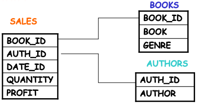
From Fact Schema to Star Schema
The conversion from a fact schema (which defines the structure of the core data) to a star schema typically involves the following steps:
Fact Table Creation: Start by creating a fact table that stores the quantitative measures and descriptive attributes associated with the fact. The fact table will contain the keys to the dimension tables and numerical measures (e.g., sales, revenue, profit).
Dimension Tables Creation: For each hierarchy or business dimension (such as time, location, or product), create a corresponding dimension table. These tables store attributes that describe the dimensions and often include a primary key for efficient indexing.
For example, consider a sales fact table that might include the following attributes:
Measures: Sales volume, profit, quantity sold.
Dimension Keys: product_key, time_key, shop_key.
Each of these keys would then link to separate dimension tables that provide more detail about the product, time, and shop. These dimension tables might include attributes like product name, category, store name, region, etc.
Guidelines for Logical Schema Design
Descriptive Attributes
Descriptive attributes provide additional information about entities within a database. For example, an attribute like “color” provides a characteristic that describes a product or a sale.
When connected to a dimension attribute: Descriptive attributes should be included in the dimension table associated with the attribute. For example, if “color” is an attribute describing a product, it should reside in the product dimension table.
When connected to a fact: If a descriptive attribute pertains directly to a fact (such as “color” associated with a sale), it should be included in the fact schema itself. This avoids unnecessary duplication and ensures that the data model reflects the connection between facts and their attributes.
Optional Attributes
Optional attributes, such as “diet” in a product catalog, are not always present for every record. In this case, introducing null values or ad-hoc placeholder values (like “N/A” or “Unknown”) is acceptable.
These attributes do not always apply to every instance in a fact or dimension table. When using null values, careful handling in queries and reports is necessary to prevent incorrect assumptions or aggregations.
Cross-Dimensional Attributes
Cross-dimensional attributes are those that define many-to-many () relationships between multiple dimensional attributes. For example, VAT might apply to both products and sales and needs to be calculated across various dimensions.
relationships: To represent such a relationship, a new table should be created that includes the cross-dimensional attribute and keys from the related dimensions. For instance, if VAT is applicable to both products and sales, the cross-dimensional attribute VAT would be included in a new table where the primary key is composed of the product and sale keys.
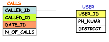
Shared Hierarchies and Convergence
A shared hierarchy refers to a hierarchy that spans across different elements of a fact table. For example, a phone call might involve both a “caller number” and a “called number,” which are conceptually different but share similar attributes (like time or duration). These two hierarchies should not be duplicated in the schema, as this would lead to unnecessary redundancy.
Same attributes with different meanings:
In this case, the shared hierarchy represents the same attributes but in different contexts. For example, “caller number” and “called number” both involve the “phone number” dimension but serve different roles in the hierarchy.
Same attributes for part of the hierarchy trees:
Here, the shared attribute might apply in one context but not the other. For instance, “city” might refer to the location of a store in one context and to the city of a customer in another.
In these cases, the bridge table is used to model the relationship between the different elements of the hierarchy. The bridge table contains the key combinations of the attributes involved in the relationship, along with the weight of each edge that represents the strength or significance of the relationship.
Bridge Tables and Multiple Edges
When there is no direct functional dependency between elements of a hierarchy, a bridge table can be introduced. This table will model the multiple edges (relationships) between the entities. The weight of each edge indicates its contribution to the cumulative relationship.
Example SQL for Profit Calculation with Weighed Queries:
In contrast, impact queries, such as counting sold copies, do not require the weight of the relationship between the entities.
Star Model and Multiple Edges
To maintain the star schema model, multiple edges can be managed by adding authors directly to the fact schema as another dimension. This approach avoids the need for weights and stores the data (like quantity and profit) directly in the fact table, linked by the appropriate dimension keys.
Secondary-View Precomputation
When designing the logical schema, particularly for materialized views, it’s important to balance various factors, including cost functions, system constraints, and user needs.
Cost Functions: Minimize the overall cost, including workload cost (i.e., the computational cost of query execution) and the cost of maintaining the materialized views (i.e., the storage and update costs).
System Constraints: These include disk space, update times, and overall system performance, all of which should be taken into consideration when deciding what views to materialize.
User Constraints: These refer to the user expectations around max answer time (how quickly queries should be answered) and data freshness (how up-to-date the data should be).
Materialized Views: When and Why
Materialized views are precomputed views that store aggregate or summary data to improve query performance. These views are useful when:
Frequent Queries: The view answers a commonly run query that is expensive to compute on the fly.
Cost Reduction: The materialized view reduces the overall cost of some queries, particularly when aggregating large volumes of data.
However, materialized views should not be created when:
The aggregation pattern is already handled by another materialized view. Creating a second view with the same pattern can lead to unnecessary redundancy.
The materialization does not significantly reduce the computational cost of queries. If the overhead of maintaining the view is greater than the benefit it provides, then it should not be materialized.