4.1 - Data Warehouses

---

Definition

A Data Warehouse (DW) is a specialized type of database designed for analytical purposes and organizational decision-making. Unlike traditional databases, which often focus on day-to-day operations, a data warehouse is characterized by several key features: it is subject-oriented, integrated, time-varying, and non-volatile.

The subject-oriented aspect means that data warehouses are organized around the major subjects of an organization, such as customers, products, sales, or finances. This organization facilitates easier analysis and reporting. The integrated nature of a data warehouse indicates that it consolidates data from various sources, ensuring consistency and compatibility across the dataset. This integration is crucial for accurate reporting and analysis, as it combines data from disparate systems into a cohesive framework.

The time-varying characteristic reflects that data in a warehouse is stored over time, enabling historical analysis. This allows organizations to observe trends, identify patterns, and make informed predictions based on past performance. Finally, the non-volatile nature of a data warehouse means that once data is entered, it remains unchanged, providing a stable environment for users to conduct analysis without worrying about fluctuations in data.

In terms of size, data warehouses can be extraordinarily large, often measured in terabytes, with many organizations managing warehouses ranging from 1 to 50 terabytes. However, some organizations, particularly those in specialized fields like Geographic Information Systems (GIS), may handle data warehouses exceeding a petabyte (1 petabyte = bytes). There are even instances of organizations dealing with exabyte (1 exabyte = bytes) and zettabyte (1 zettabyte = bytes) data volumes, such as national medical records or large-scale weather data, respectively.

Data Warehouses vs. Data Lakes

The concept of data storage extends beyond data warehouses to include data lakes, also referred to as dataspace. While both serve the purpose of data storage and analysis, they differ significantly in structure and application. A data warehouse typically uses a relational database management system (RDBMS), emphasizing the storage of structured data that is recognized as having high value. In contrast, data lakes often utilize distributed file systems, such as Hadoop Distributed File System (HDFS), which allows for the storage of a wider variety of data types, including structured, semi-structured, and unstructured data.

In a data warehouse, data is usually aggregated and transformed to conform to enterprise standards before it is stored. This approach ensures that users are working with consistent, high-quality data but requires upfront data integration efforts. Conversely, data lakes prioritize fidelity to the original format, enabling organizations to store raw data without immediate transformation. This flexibility allows users to integrate and analyze data on demand, which can be particularly valuable for exploratory data analysis.

Furthermore, data warehouses operate on a “schema-on-write” principle, meaning that the schema is defined before data is written to the database. This pre-defined structure is useful for ensuring data integrity and performance. In contrast, data lakes utilize a “schema-on-read” approach, where the schema is applied only when data is accessed for analysis. This flexibility accommodates diverse analytical needs but can lead to complexities in data retrieval and analysis.

Feature	Data Warehouse	Data Lake
Data Structure	Structured data	Structured, semi-structured, and unstructured data
Storage Technology	Relational Database Management System (RDBMS)	Distributed file systems (e.g., Hadoop Distributed File System - HDFS)
Schema	Schema-on-write (schema defined before data is written)	Schema-on-read (schema applied when data is read)
Data Processing	Data is cleaned, transformed, and integrated before storage	Raw data is stored in its original format
Use Case	Historical analysis, reporting, and business intelligence	Exploratory data analysis, big data processing, and machine learning
Data Quality	High-quality, consistent data	Variable data quality, as raw data is stored without transformation
Performance	Optimized for complex queries and read operations	Optimized for large-scale data storage and processing

Differences Between Transactional Databases and Data Warehouses

Most data warehouses are stored within RDBMS, but they represent a specialized type of database that requires different operations compared to traditional transactional databases. The distinctions between these two systems can be categorized based on their processing types: Online Transactional Processing (OLTP) for transactional databases and Online Analytical Processing (OLAP) for data warehouses.

Transactional Databases (OLTP)

Transactional databases are primarily designed for managing and processing high volumes of transactions efficiently. They focus on rapid updates and data integrity, serving the day-to-day operational needs of an organization. Typically, OLTP systems handle many small transactions that are often short and straightforward, such as inserting, updating, or deleting records. These operations are crucial for tasks like order processing, inventory management, and customer relationship management.

The data stored in transactional databases usually ranges from gigabytes (GB) to petabytes (PB), accommodating the daily transactions generated by an organization. The emphasis is on maintaining a current snapshot of data, which reflects the most recent state of operations. To ensure quick access and efficient processing, OLTP systems use indexing and hashing techniques based on primary keys, allowing for fast retrieval of records. Transactional databases typically support thousands of users, primarily generic employees who require access to operational data for their daily tasks.

Data Warehouses (OLAP)

In contrast, data warehouses are tailored for complex analysis and reporting, making them ideal for strategic decision-making. They predominantly focus on reading data rather than updating it. Queries in a data warehouse tend to be long and complex, designed to extract meaningful insights from vast datasets. As a result, data warehouses often handle much larger volumes of data, typically in the range of petabytes to exabytes, accommodating extensive historical data for analysis.

While transactional databases capture a current snapshot of data, data warehouses store historical information, enabling organizations to track trends and patterns over time. The data in a warehouse is summarized and reconciled, providing a more cohesive view of the information. This summarized data is critical for generating reports, performing advanced analytics, and conducting business intelligence activities.

Data warehouses rely heavily on data scans rather than indexing, as the analytical queries often require examining large datasets to uncover insights. Users of data warehouses are typically more limited in number (often in the hundreds) and include company management and analysts who require in-depth analysis for informed decision-making.

The Utility of Data Warehouses Across Industries

Data warehouses are essential for consolidating data from multiple sources and enabling complex analyses, supporting informed decision-making and strategic planning across various sectors.

• Commerce: Data warehouses help retail and e-commerce businesses analyze sales and customer feedback, identify trends, and optimize shipping and stock control, leading to improved customer satisfaction and efficient supply chain management.
• Manufacturing Plants: In manufacturing, data warehouses monitor production processes, manage costs, and support order management and inventory control, allowing for better resource allocation and production planning.
• Financial Services: Financial institutions use data warehouses for risk assessment and fraud detection by analyzing credit card transactions and aggregating historical data related to loans and investments, aiding in creditworthiness and risk management.
• Telecommunications: Telecom providers analyze call flow and subscriber profiles using data warehouses to assess network performance, identify usage patterns, and enhance customer service through targeted marketing and personalized services.
• Healthcare Structures: Healthcare organizations utilize data warehouses to track patient flows, understand treatment costs, and improve resource allocation, enhancing operational efficiency and patient care through informed decision-making.

Architecture of a Data Warehouse

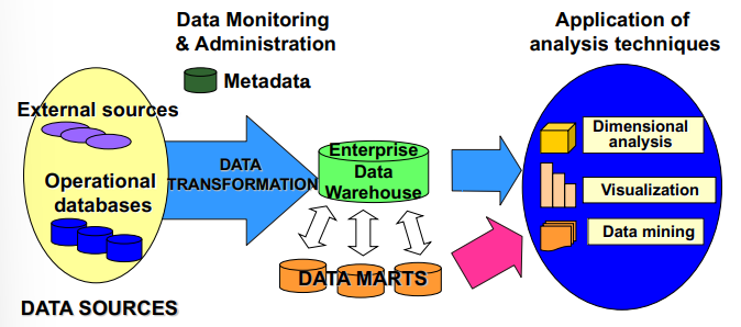
The architecture of a data warehouse is designed to support complex data analysis and decision-making processes by organizing and transforming large volumes of data into an accessible format. The following components outline the typical architecture of a data warehouse:

At the core of the data warehouse architecture are data sources, which provide the raw data that will be processed and analyzed. These sources can include external sources, such as third-party data providers, and operational databases within the organization. Operational databases store transactional data from daily operations, such as sales records, customer interactions, and inventory data. This raw data from multiple sources is fed into the data warehouse for further processing.

Once data is collected from various sources, it goes through a data transformation process. This phase involves cleaning, normalizing, and integrating data from different systems to ensure consistency and accuracy. Data from disparate sources must be converted into a unified format to enable accurate analysis. The transformation process includes tasks such as resolving data conflicts, handling missing data, and applying business rules. After transformation, the data is ready to be loaded into the data warehouse.

The Enterprise Data Warehouse (EDW) serves as the central repository for all the integrated data within the organization. It contains historical and current data that has been processed and organized for analytical purposes. The EDW is structured to support queries, reporting, and analysis, making it a key element in an organization’s data strategy. Data within the EDW is often aggregated and summarized, providing a comprehensive view of the organization’s operations.

Definition

Data Marts are smaller, specialized databases within the overall data warehouse architecture. They contain subsets of data that are tailored to the needs of specific departments or business units, such as finance, marketing, or sales. Data marts allow users to access relevant data quickly without querying the entire data warehouse.

These departmental data stores provide a more focused and efficient means of accessing specific data for targeted analysis.

Data stored in the EDW and data marts can be accessed through various analytical techniques. Some key analysis methods include:

• Dimensional analysis, which allows users to view data from multiple perspectives, such as by time, product, or region.
• Data mining, a process that uses algorithms to discover patterns, trends, and relationships within the data.
• Visualization tools, which help present data in an understandable format, such as charts, graphs, or dashboards. These tools make it easier for decision-makers to interpret complex data.

An essential part of maintaining a data warehouse is data monitoring and administration. This ensures the smooth functioning of the system, manages performance, and maintains data quality. Metadata provides information about the data stored in the warehouse, such as its structure, source, and lineage. Metadata helps users understand the context of the data and facilitates data governance.

The Role of Big Data in Relation to Data Warehouses

With the rise of Big Data technologies, many organizations wonder whether data warehouses are becoming obsolete. However, big data infrastructures, such as cloud-based data lakes or distributed systems like Hadoop, are not intended to directly replace data warehouses. Instead, these two technologies are complementary and serve distinct purposes.

A data warehouse is more than just a storage system; it represents a paradigm for organizing, processing, and analyzing structured data, usually in a relational database management system. It focuses on integrating, cleaning, and transforming data upfront, making it ideal for structured and historical data analysis.

On the other hand, Big Data technologies are designed to handle vast volumes of unstructured or semi-structured data, such as text, social media, sensor data, or multimedia. These technologies allow organizations to store raw data in its original format, applying analysis and transformation on demand. Big data infrastructures are often more flexible and scalable than traditional data warehouses, but they typically lack the rigorous data integration and summarization processes that define data warehousing.

That said, cloud-based repositories can house data warehouses, offering scalability and flexibility without sacrificing the structured nature of the data. This enables organizations to benefit from the strengths of both paradigms—using data warehouses for structured, historical analysis while leveraging big data infrastructures for handling large volumes of diverse data.

Examples of Data Warehouse Queries

The capabilities of a data warehouse are often demonstrated through complex queries designed to provide insights from large datasets. Below are examples of common queries used in data warehouses:

1. Sales Aggregation Query: “Show total sales across all products at increasing aggregation levels for a geographic dimension, from state to country to region, for the years 1999 and 2000.” This type of query enables users to analyze sales performance at different geographic levels, helping organizations understand regional market dynamics and trends over time.

2. Cross-Tabular Analysis of Expenses: “Create a cross-tabular analysis of our operations showing expenses by territory in South America for 1999 and 2000. Include all possible subtotals.” This query provides a detailed breakdown of operational expenses, offering insights into cost control and financial performance across different territories.

3. Top Sales Representatives Ranking: “List the top 10 sales representatives in Asia according to sales revenue for automotive products in the year 2000, and rank their commissions.” This query helps management identify high-performing sales representatives and evaluate their commissions, aiding in performance reviews and incentive planning.

Logical Models for OLAP: The Data Cube Metaphor

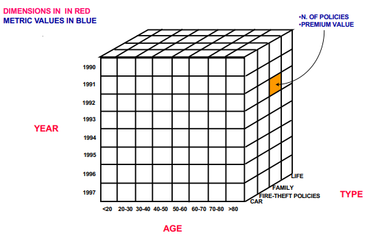
In Online Analytical Processing (OLAP), data is typically modeled in a data cube format, which allows for efficient multi-dimensional analysis. The data cube metaphor provides a way to visualize and represent data across various dimensions, facilitating complex queries and computations. Each axis or dimension of the cube represents a different aspect of the data, such as time, product type, or customer demographics. The cells within the cube contain metric values, such as the number of policies sold or premium values in the case of an insurance company.

Example: Insurance Company Data Cube

Consider an insurance company analyzing its policies over different dimensions:

• Dimensions: The main dimensions for analysis in this case could be age, year, and policy type.
  • Age represents different age groups of policyholders.
  • Year captures the temporal aspect, ranging from 1990 to 1997.
  • Type represents the type of policy, such as car insurance, fire-theft policies, family policies, or life insurance.
• Metric Values: Within each cell of the cube, metric values such as the number of policies or the premium value are stored, providing insight into how many policies were sold or the total premiums collected for specific combinations of age group, year, and policy type.

To support sophisticated analyses, OLAP-oriented data models are structured to handle multi-dimensional data efficiently. The most suitable representation for OLAP is the data cube, where:

• Cube dimensions act as search keys, enabling queries based on specific aspects such as time or product.
• Dimensions can be hierarchical, allowing for different levels of granularity in the analysis. For instance, a time dimension might be broken down into DAY-MONTH-TRIMESTER-YEAR, and a product dimension might be represented as BRAND-TYPE-CATEGORY (e.g., LAND ROVER → CARS → VEHICLES).
• Cube cells contain metric values (e.g., sales figures, number of transactions), which are the focus of analysis.

Typically, data cube models are implemented over a relational DBMS, providing flexibility in querying and analysis.

Dimensional Fact Model (DFM)

The Dimensional Fact Model (DFM) is a logical model used to describe the structure of data cubes in more detail. It defines how facts, measures, and dimensions are related, and helps to organize data for efficient OLAP querying.

Definition

• Facts: A fact is a concept that represents events or transactions relevant to the decision-making process. In a business setting, facts usually correspond to specific occurrences, such as sales, phone calls, or insurance policies issued.
• Measures: A measure is a numerical attribute of a fact. For example, in an insurance data cube, the measures could include the number of policies sold or the premium value.
• Dimensions: A dimension is an attribute of a fact that serves as a coordinate for analysis. Dimensions allow users to slice and dice the data across different perspectives, such as time, location, or product category.
• Dimension Hierarchies: Dimensions can often be broken down into hierarchical levels. For instance, in a time dimension, you might analyze data by day, month, quarter, or year, enabling flexible and granular analysis.

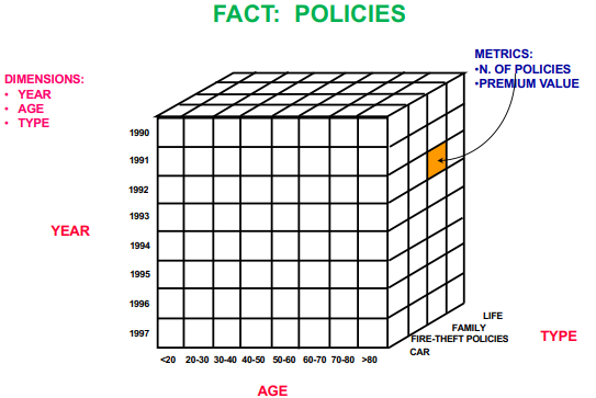
Example: Insurance Company Data Cube

Let’s break down the components of an insurance company’s data cube:

• Fact: The fact is Policies, representing the number of insurance policies sold.

• Measures:

  • Number of policies sold.
  • Premium value, which represents the total amount collected for each policy type.

• Dimensions:

  • Year: Temporal dimension, capturing the years from 1990 to 1997.
  • Age: Age groups of policyholders, categorized into bands.
  • Policy Type: The type of insurance policy (e.g., car, fire-theft, family, life).

This structure allows the insurance company to perform complex analyses, such as examining how the number of car policies for individuals in the 30-40 age group has changed over the years or comparing premium values between different age groups for life insurance policies.

Other Examples of Data Cube Applications

Store Chain

• Fact: Sales transactions.
• Measures:
  • Sold quantity: The number of units sold for a given product.
  • Gross income: The total revenue generated from sales.
• Dimensions:
  • Product: The items sold in the store.
  • Time: The date or time period when the sales occurred.
  • Zone: The geographic location of the store or the sales region.

Telecom Operator

• Fact: Phone calls made by subscribers.
• Measures:
  • Cost: The amount charged for the call.
  • Duration: The length of the phone call.
• Dimensions:
  • Caller subscriber: The person initiating the call.
  • Called subscriber: The person receiving the call.
  • Time: The time period when the call took place.

Multidimensional Representation in Sales Analysis

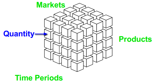
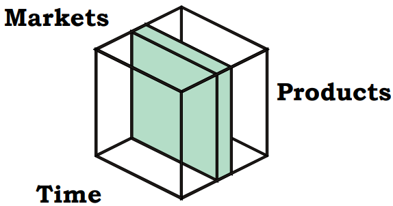
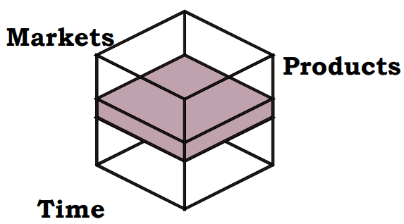
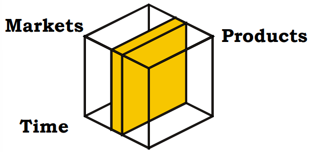
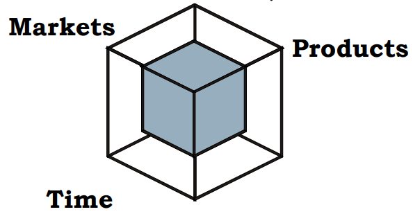
In a sales analysis context, a sales cube provides a multidimensional representation of data, allowing managers and analysts to examine and interpret sales performance across various dimensions such as products, time periods, and markets. This approach enables different stakeholders within an organization to focus on specific aspects of the sales data that are most relevant to their roles.

The sales cube can be conceptualized as comprising three primary dimensions:

1. Products: This dimension includes the various products sold by the company. Each product can be further categorized into subcategories, such as product types, brands, or other classifications.
2. Time Periods: This dimension captures the temporal aspects of sales data. It can be structured hierarchically to include days, months, quarters, and years, allowing for different levels of temporal analysis.
3. Markets: The market dimension represents different geographical or demographic markets where the products are sold. This can include various levels of granularity, such as individual stores, cities, regions, or larger market areas.

Use Cases for Different Managers

Different managers can analyze the sales cube from various perspectives, tailored to their specific interests and responsibilities:

• Area Manager: The area manager may focus on the sales performance of products within their own markets. This analysis allows them to evaluate how different products are performing in their specific areas and make informed decisions about inventory and marketing strategies.

  

• Product Manager: The product manager can examine the sales of a specific product across all time periods and markets. This comprehensive analysis helps them understand the product’s overall performance, identify trends, and adjust marketing strategies accordingly.

  

• Financial Manager: The financial manager might concentrate on product sales across all markets for the current period and the previous one. This analysis provides insights into revenue fluctuations and helps assess financial performance over time.

  

• Strategic Manager: The strategic manager can focus on a category of products within a specific region and a medium-term time span. This approach allows them to develop strategies that capitalize on market opportunities and align with broader organizational goals.

  

In addition to the main dimensions, each dimension can have hierarchical structures that facilitate more granular analysis. For instance:

• Market Dimension
• Time Dimension
• Product Dimension

graph TD
    subgraph 1[Market Dimension]
        direction BT
        store --> city --> reg.area --> region
    end

    subgraph 2[Time Dimension]
        direction BT
        day --> month --> trimester --> year
    end

    subgraph 3[Product Dimension]
        direction BT
        product --> category 
        product --> brand
    end

Aggregate Queries Over Hierarchies

Using the hierarchical structures, analysts can execute various aggregate queries to gain insights from the sales cube. Here are some examples:

1. Total sales per product category, per supermarket, per day:
   This query allows managers to assess daily sales performance across different product categories and supermarkets, identifying trends and opportunities for growth.
2. Total monthly sales for all products, per supermarket:
   This query aggregates sales data by month for all products sold in each supermarket, offering a broader view of performance trends over time.
3. Total monthly sales per category, per supermarket:
   By analyzing total monthly sales by category for each supermarket, managers can determine which categories are driving sales in different locations.
4. Average monthly sales per category, for all supermarkets:
   This query provides insights into overall category performance across all supermarkets, allowing for comparisons and performance benchmarks.

OLAP Operations

Online Analytical Processing provides a set of operations that enable users to analyze data from multiple perspectives efficiently. These operations allow for various types of data manipulations and insights, which are crucial for effective decision-making. Here are the main OLAP operations:

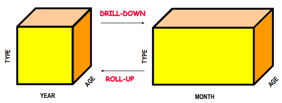
1. Roll-Up: This operation aggregates data at a higher level of granularity. For example, it can summarize last year’s sales volume by product category and region. By moving up the hierarchy (e.g., from months to quarters or from specific products to categories), users can obtain a broader view of performance.

2. Drill-Down: The drill-down operation de-aggregates data, allowing users to examine it at a more detailed level. For instance, if a user wants to analyze sales for a specific product category and region, they might drill down to see daily sales figures. This operation helps identify trends and patterns that may not be visible at higher aggregation levels.

   

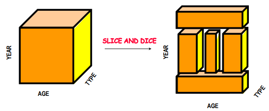
3. Slice-and-Dice: This operation involves applying selections and projections to reduce the dimensionality of the data. For example, a user may select a specific time period and product category to analyze, effectively “slicing” the cube to focus on relevant data. “Dicing” allows further analysis by choosing different dimensions or metrics, providing flexibility in exploration.

   

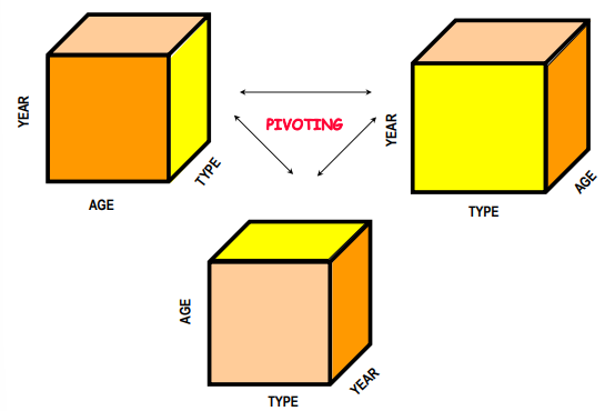
4. Pivoting: Also known as rotation, pivoting re-orients the data cube by selecting two dimensions to re-aggregate the data. This operation allows users to view the same data from different angles, facilitating comparative analysis across different dimensions.

   

5. Ranking: The ranking operation sorts data according to predefined criteria, allowing users to quickly identify top-performing entities. For example, a user might rank products based on sales revenue or growth percentage, enabling strategic decisions based on performance metrics.

6. Traditional Operations: These include standard database operations such as select, project, join, and the creation of derived attributes. These operations are foundational to OLAP and are often used in conjunction with the more specialized OLAP operations mentioned above.

Visualization and Reports

The results of OLAP operations can be visualized in various formats to enhance understanding and communication of data insights. Visualization options may include:

• Tables: Organize data into rows and columns for easy comparison.
• Histograms: Display frequency distributions to highlight patterns.
• Graphics: Use charts (bar, line, pie) to represent data visually, making trends and comparisons clearer.
• 3D Surfaces: Provide a more interactive and immersive experience for analyzing multidimensional data.

Using these visualization techniques, users can create reports that are not only informative but also visually appealing, aiding in the interpretation of complex data sets.

OLAP Logical Models

OLAP systems can be categorized into different logical models, each with its own approach to storing and processing data:

1. MOLAP (Multidimensional On-Line Analytical Processing): MOLAP utilizes a multidimensional data structure, often referred to as a “physical” data cube. This model is optimized for rapid data retrieval and is particularly effective for complex queries. The multidimensional array format allows for efficient aggregations and computations across various dimensions.
2. ROLAP (Relational On-Line Analytical Processing): ROLAP employs the relational data model to represent multidimensional data. This approach is widely adopted because it leverages existing relational database technologies, making it easier to integrate with current systems. ROLAP systems use SQL to query data, often creating views to represent multidimensional aspects.

A New SQL Operation: The Data Cube

The introduction of a new SQL operation called the data cube allows for the expression of all possible tuple aggregations from a table. This operation enhances the ability to perform complex aggregations and provides a comprehensive view of the data.

The data cube operation uses a new polymorphic value, ALL, which represents the need for aggregation across multiple dimensions. In some systems, NULL may be used instead to indicate similar aggregative functions. This capability makes it easier for analysts to generate reports that include all combinations of data points, facilitating a more thorough understanding of the relationships within the data.

Example of Data Cube Instruction in SQL (ROLAP)

The following SQL query demonstrates how to use the CUBE operator in a relational OLAP context to generate a data cube that aggregates sales data for specific car models over a specified time period:

SELECT Model, Year, Color, SUM(Sales)
FROM Sales
WHERE Model IN ('Fiat', 'Ford')
  AND Color = 'Red'
  AND Year BETWEEN 1994 AND 1995
GROUP BY (Model, Year, Color)
WITH CUBE;

Consider the following table representing sales data:

Model	Color	Year	Sales
Fiat	Red	1994	50
Fiat	Red	1995	85
Ford	Red	1994	80

When executing the query with the CUBE operator, the result includes all possible aggregations, as shown in the following table:

Model	Color	Year	Sum (Sales)
Fiat	Red	1994	50
Fiat	Red	1995	85
Fiat	ALL	1994	50
Fiat	ALL	1995	85
Fiat	Red	ALL	135
Fiat	ALL	ALL	135
Ford	Red	1994	80
Ford	ALL	1994	80
Ford	Red	ALL	80
Ford	ALL	ALL	80
ALL	Red	1994	130
ALL	Red	1995	85
ALL	Red	ALL	215
ALL	ALL	1994	130
ALL	ALL	1995	85
ALL	ALL	ALL	215

The table above illustrates how the CUBE operator generates a comprehensive view of the data, allowing users to analyze sales figures across different dimensions and levels of aggregation.

Roll-Up Operation

The ROLLUP operator enables a SELECT statement to compute multiple levels of subtotals across specified group dimensions. Unlike the CUBE operator, which evaluates all combinations of columns, ROLLUP performs aggregations in a hierarchical manner, essentially offering a “progressive aggregation.”

Here is how the ROLLUP SQL statement looks:

SELECT Model, Year, Color, SUM(Sales)
FROM Sales
WHERE Model IN ('Fiat', 'Ford')
  AND Color = 'Red'
  AND Year BETWEEN 1994 AND 1995
GROUP BY (Model, Year, Color)
WITH ROLLUP;

The output after applying the ROLLUP operator can be seen in the table below:

Model	Color	Year	Sum (Sales)
Fiat	Red	1994	50
Fiat	Red	1995	85
Ford	Red	1994	80
Fiat	ALL	1994	50
Fiat	ALL	1995	85
Ford	ALL	1994	80
Fiat	ALL	ALL	135
Ford	ALL	ALL	80
ALL	ALL	ALL	215

In this table, the ROLLUP operator has generated subtotals for each model and color combination, as well as overall totals for the selected dimensions.

The key difference between the CUBE and ROLLUP operators lies in their approach to aggregation:

• CUBE evaluates aggregate expressions across all possible combinations of the columns specified in the GROUP BY clause. It provides a more extensive view, allowing for multifaceted analysis.
• ROLLUP, on the other hand, evaluates aggregate expressions relative to the hierarchical order of the columns specified in the GROUP BY clause. This means that it provides subtotals in a more structured way, focusing on higher levels of aggregation without calculating all possible combinations.