graph TD
	UR((User<br>Requirement))
    DBs((Internal<br>DBs))
    IS((Further<br>Info Sources))
    SS[Source Selection]
    TA[Translation into a<br>common conceptual model]
    SA[Source Analysis]
    CS[Conceptual Schema<br>integration]
    CD[Conceptual Design]
    LD[Logical Design]
    PD[Physical Design]

    UR --> SS
    DBs --> SS
    IS --> SS

    subgraph Analysis
        direction LR
        SS --> TA
        TA --> SA
    end

    subgraph Integration
        SA --> CS
    end

    subgraph Design
        direction LR
        CS --> CD
        CD --> LD
        LD --> PD
    end
In data warehousing, the conceptual design phase is critical for developing a high-level, structured representation of the integrated database. This phase involves carefully documenting the main schema types that will guide the subsequent design stages. In particular, the conceptual design focuses on two main types of schemas:
-
Conceptual Schema: This schema defines the essential structure of the data warehouse independently of any physical implementation. It typically uses models such as the Entity-Relationship (E/R) model or UML class diagrams to represent the core entities, their attributes, and the relationships between them. Through these diagrams, the conceptual schema provides a foundational overview of how different data elements interact conceptually, without focusing on the specific storage or access methods that will be used later.
-
Logical Schema: Once the conceptual schema is established, the logical schema provides a more detailed representation of the data structure, mapping it to specific formats that align more closely with the database technologies. This schema could be in a relational format (for traditional relational databases) or in XML format (for hierarchical or document-oriented data stores). While the logical schema is still independent of physical storage details, it represents the data structure in a way that is understandable for database management systems, enabling a more streamlined translation to the physical implementation stage.
The design process for a data warehouse often follows a top-down methodology, which begins with the selection of facts and then incrementally defines the associated dimensions and measures. This approach ensures that the data warehouse design remains focused on business needs and analytical goals. The top-down methodology can be broken down into the following stages:
-
Fact Choice (Subject-Oriented Focus) The first step in the top-down methodology is choosing the facts, or primary data entities, that are relevant to the business domain. Facts represent key business processes or events and are subject-oriented, meaning they are chosen based on the main topics or subjects of analysis within the organization. Examples of typical facts might include sales transactions, customer interactions, or inventory levels, each corresponding to a distinct business activity that is important for analysis.
-
Attribute Tree Design for Each Fact Once the primary facts are defined, each fact undergoes further analysis to identify the attributes associated with it. An attribute tree is created to illustrate the hierarchical structure of these attributes, organizing them from the most general to the most specific. For instance, a sales fact might have attributes such as time of transaction, product category, and store location. The attribute tree visually represents how these attributes are related and organized within the data structure.
-
Attribute-Tree Editing After establishing an initial attribute tree, it is refined through a process called attribute-tree editing. This stage involves reviewing and modifying the tree to ensure that all attributes are relevant, non-redundant, and accurately represent the fact in question. Any ambiguities or redundancies are addressed, and the tree is adjusted to enhance clarity and logical consistency, ultimately improving the data warehouse’s effectiveness in supporting analysis.
-
Dimension Definition Dimensions are then defined based on the attributes in the tree. Dimensions are categories of data that provide context to the facts, allowing for multi-dimensional analysis. For example, a sales fact might have dimensions such as time, geography, and product, enabling users to view sales data across various time periods, regions, or product categories. This step ensures that the data warehouse is designed to facilitate slicing, dicing, and drilling down through data along relevant dimensions.
-
Measure Definition Measures are quantitative values associated with each fact that can be analyzed along the defined dimensions. In the case of a sales fact, measures might include quantities sold, revenue, or profit. Each measure is designed to be meaningful for analysis and provides numerical insights into the fact’s performance. Defining measures involves specifying their calculation rules, aggregation levels, and any additional information needed to interpret them accurately.
-
Fact Schema Creation Finally, a fact schema is created to encapsulate the relationships between facts, dimensions, and measures. This schema, often implemented as a star or snowflake schema in the physical data warehouse, serves as a blueprint for how the data will be structured, stored, and retrieved. The fact schema ensures that data can be efficiently queried and analyzed across multiple dimensions, supporting the data warehouse’s role as a robust analytical resource for the organization.
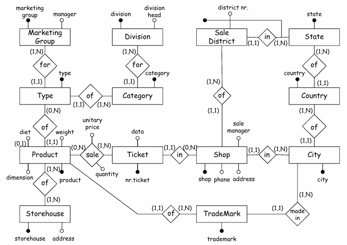
Consider the following relational schema about a company that sells products in different shops:
Product(product, weight, dimension, trademark:TradeMark, type:Type)
Shop(shop, address, phone, salemanager, (district, state):District, city:City)
Ticket(nrticket, date, shop:Shop)
Sale(product:Product, nrticket:Ticket, quantity, unitaryprice)
Storehouse(storehouse, address)
City(city, country:Country)
Country(country, state:State)
State(state)
District(district, state:State)
Prod_Storehouse(product:Product, storehouse:Storehouse)
TradeMark(trademark, madein:City)
Type(type, marketinggroup:MarketingGroup, category:Category)
MarketingGroup(marketinggroup, manager)
Category(category, division:Division)
Division(division, divisionhead)
We start from the corresponding E/R schema
Fact definition
In data warehousing, defining facts is a foundational step in organizing data for analysis, as facts represent key events or transactions that occur dynamically within an organization. Facts are central to the analytical processes within a data warehouse because they capture business activities, often through metrics or quantitative information, which can then be analyzed over time.
Facts correspond to events or transactions that occur within the business environment and are essential to the organization’s analytical goals. In an Entity-Relationship schema, a fact can correspond to a specific entity (denoted as
For a fact to be considered a “good candidate” in a data warehouse, it should ideally represent entities or relationships that are frequently updated within the organization, such as “sales” or “orders.” These facts are suitable for a data warehouse because they capture dynamic, time-sensitive information that can reveal trends and patterns. On the other hand, static archives, which do not change frequently, are generally not suitable as facts in a data warehouse. Since data warehouses are designed to analyze changes and trends over time, static data lacks the evolving nature that is essential for dynamic analysis.
When a fact is identified for study, it becomes the “root” of the fact schema. The fact schema is a structured way of organizing facts and their associated dimensions and measures, supporting a logical and efficient approach to data analysis.
Defining the Attribute Tree
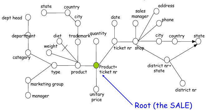
The attribute tree is a hierarchical representation of the attributes related to a fact, organizing them in a way that reflects their dependencies and relationships. In an attribute tree, each node represents an attribute that is either simple (e.g., a single data field) or complex (e.g., a composite attribute with multiple components) as defined in the source schema.
-
The Root Node in an attribute tree corresponds to the primary key of the fact being analyzed. This root uniquely identifies instances of the fact and serves as the central point of reference for all related attributes in the tree.
-
Each Node in the attribute tree functionally determines its descendant attributes, meaning that each node’s value dictates the values of the attributes directly below it in the hierarchy. This structure captures how attributes are interrelated, helping to define dependencies and optimize data retrieval for analysis.
To build the attribute tree, a semi-automated procedure can be used, often starting with the E/R schema of the source data. This process involves mapping entities and relationships from the E/R model onto the attribute tree, transforming complex data structures into an organized, hierarchical model that mirrors the dependencies within the data. This approach allows data architects to systematically capture the structure of the source data and adapt it for analysis within the data warehouse. By organizing attributes in this manner, the attribute tree becomes a pivotal structure for ensuring that data can be navigated efficiently when creating dimensional models and conducting multi-dimensional analysis.
Attribute Tree Editing
In data warehouse design, the attribute tree serves as a structured representation of the attributes associated with a specific fact.
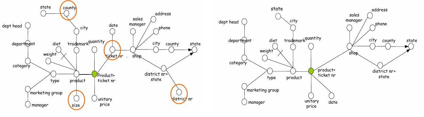
The editing phase of the attribute tree is crucial for optimizing the tree for analytical efficiency. This stage allows designers to refine the tree by removing any irrelevant attributes that do not add value to the specific data mart. Editing techniques include pruning and grafting, which help streamline the attribute tree by focusing on the most relevant data for analysis:
Definition
Pruning involves removing a node
and its entire subtree, which is all the attributes hierarchically dependent on . This process is particularly useful when certain attributes within a subtree do not contribute to the data mart’s objectives. Grafting is another editing approach, where a node
is removed, but its child nodes are connected directly to ’s parent node. This preserves the information in the subtree but simplifies the hierarchy, making it easier to manage and navigate.
Special Cases in Attribute Tree Editing
Certain complex structures, such as cyclic relationships, ISA hierarchies, and compound attributes, require additional consideration during attribute tree editing. These structures introduce challenges that need to be addressed for the data warehouse schema to remain effective and usable:
-
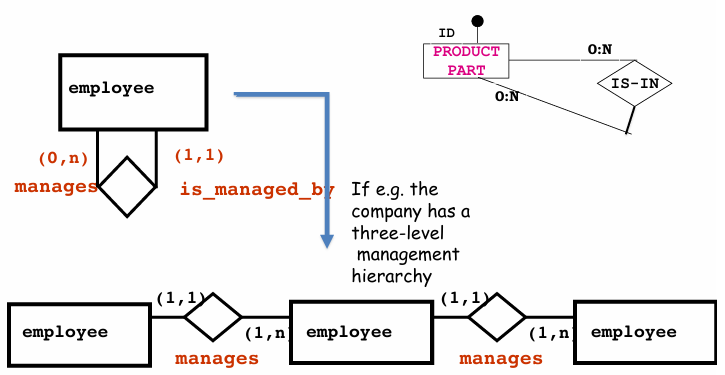
Cyclic Relationships: Cyclic relationships, such as a part-subpart hierarchy or an employee-manager reporting structure, occur when an entity relates back to itself in a loop. In a scenario like a three-level management hierarchy, this could create a cycle in the attribute tree. To handle these cycles, they must be carefully broken at a defined point in the hierarchy. For example, an employee-manager hierarchy could be restricted to a specific number of levels, such as three, to avoid infinite recursion and simplify the analysis process.
-
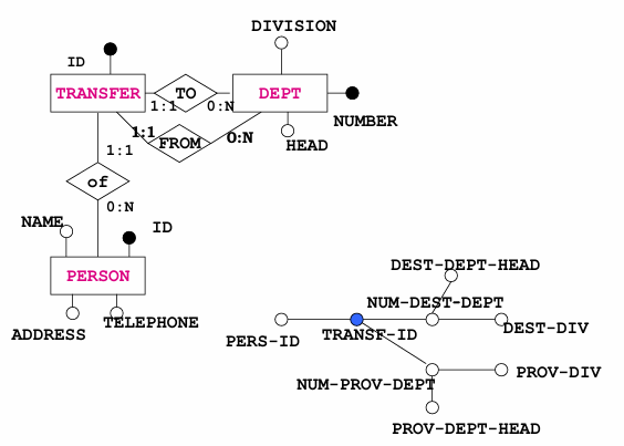
Cycles in the Schema: In cases where the original schema contains cycles, these cycles must also be broken to avoid redundancy and confusion in the data warehouse. One approach is to select the most logical or convenient link within the cycle to retain, breaking the rest of the loop to create a more linear structure. This helps maintain clarity in the attribute tree and improves performance by reducing complexity.
-
IS_A Hierarchies: In entity-relationship modeling, IS_A hierarchies represent inheritance, where one entity type is a specialization of another. For instance, an “employee” entity might have subtypes like “manager” or “technician.” These ISA hierarchies are treated like optional (
) relationships in the attribute tree, enabling flexible inclusion of specific attributes from the hierarchy as needed without creating redundant links. 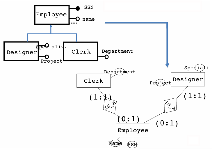
-
Compound Attributes: Attributes that consist of multiple components, such as a full address (with street, city, state, and zip code), are treated as compound attributes. These attributes are represented as a vertex with child nodes corresponding to each component, allowing the attribute tree to capture the detailed structure of compound data elements while still representing them within a single logical grouping.
Each of these special cases requires careful handling to maintain the logical flow and usability of the attribute tree. By managing complex relationships and editing out non-essential attributes, the attribute tree can be streamlined to serve as an efficient, insightful structure for supporting the data mart’s analytical objectives.
Dimension Definition
Dimensions are key attributes that provide context to the facts within a data warehouse, enabling users to analyze data across different perspectives or “dimensions.” In the attribute tree, dimensions are typically selected from the attributes that are direct children of the root node, which represents the primary fact being analyzed.
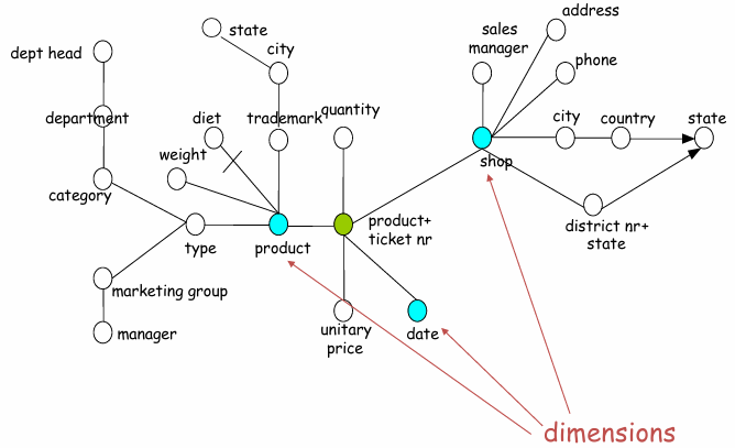
The time dimension is universally important in data warehousing because it allows for the analysis of trends over different time periods.
If the data source is historical—where each record captures data over time—then time can be directly mapped as a dimension. However, if the source is a snapshot (i.e., capturing a single moment in time without historical depth), then a time dimension may need to be artificially added. This can involve timestamping records or adding calendar-related attributes to enable time-based analysis.
Measure Definition
Measures are quantitative attributes associated with the fact, providing numerical insights that can be analyzed through various operations. While dimensions categorize the fact, measures quantify it. In an attribute tree, measures are usually derived from numerical attributes of the root fact. For example, in a sales model, unitary price or quantity sold can act as measures. Measures often become more meaningful when aggregate functions are applied, allowing for deeper insights through calculations such as totals, averages, and counts.
Common aggregate functions include:
- Sum: Useful for calculating total values, such as total sales.
- Average: Useful for determining average values, such as average unit price.
- Min and Max: Useful for identifying the smallest or largest value in a dataset, such as minimum and maximum sales amounts.
- Count: Useful for determining the frequency of occurrences, such as the number of sales transactions.
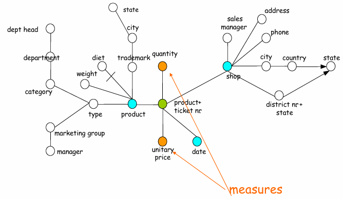
For example, specific measures could be defined as follows:
- Quantity Sold: Defined as
SUM(Sale.quantity), representing the total quantity of products sold. - Gross Income: Defined as
SUM(Sale.quantity * Sale.unitaryprice), calculating the total income generated from sales. - Average Price: Defined as
AVG(Sale.unitaryprice), giving insight into the average selling price of items. - Number of Tickets: Defined as
COUNT(*), indicating the total number of sales transactions or tickets.
It is also possible for a fact to have no measures, especially if it serves more as a categorical reference than a quantitative one. Additionally, if the granularity (the level of detail) of a fact differs from that of the source schema, creating measures can be essential for aggregating data appropriately. This helps align data from different granularities, allowing for flexible analysis at multiple levels (e.g., daily, monthly, or yearly summaries).
Glossary and Expressions for Measures
A glossary is often maintained within the data warehouse schema, associating a clear definition or formula with each measure. This glossary provides a reference for how each measure is calculated across various levels of aggregation, helping users understand the source of each metric and its computation at different hierarchical levels. By clearly defining these expressions, the data warehouse ensures consistency in metric calculation and clarity in analytical processes.
For example:
- Quantity: Calculated using the expression
SUM(Sale.quantity). - Gross Income: Derived from
SUM(Sale.quantity * Sale.unitaryprice). - Unitary Price: Averaged using
AVG(Sale.unitaryprice). - Number of Tickets: Determined by
COUNT(*).
Each expression encapsulates how measures are calculated and aggregated, thus providing a clear and consistent understanding of each metric for analysts. This organized approach ensures that measures are readily interpretable, accurately computed, and aligned with the organization’s reporting and analytical needs.
Fact Schema Creation
In data warehousing, fact schema creation is the process of translating the attribute tree into a structured schema that organizes facts along with their dimensions and measures. This schema is essential for enabling the multi-dimensional analysis of data, allowing users to explore and understand relationships and patterns within the data warehouse.
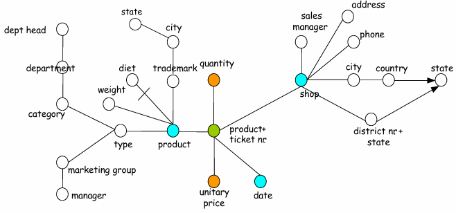
The attribute tree serves as the starting point for fact schema creation. In this process, the hierarchical structure of the attribute tree is mapped to form the fact schema, incorporating both dimensions (categorical attributes that contextualize the fact) and measures (quantitative attributes that provide meaningful metrics). The resulting schema represents how data will be stored and accessed in the warehouse, with dimensions and measures organized in a way that facilitates querying and reporting.
Dimension Hierarchies
Each dimension hierarchy within the fact schema corresponds to a subtree within the attribute tree, where each subtree’s root represents a unique dimension. Dimension hierarchies organize data into levels, from the most granular (fine detail) to the least granular (summary levels). For instance, in a sales schema, the “Location” dimension hierarchy might include levels such as store, city, and region, allowing users to analyze sales data across different geographic levels. Similarly, a “Time” dimension could include levels like day, month, and year.
These hierarchies allow for drill-down and roll-up analyses, enabling users to view data at both granular and summarized levels. The organization of dimension hierarchies within the fact schema makes it possible to perform complex analytical queries, examining trends and patterns at multiple levels of detail.
Naming the Fact Schema
The name of the fact schema generally corresponds to the name of the main entity or event being analyzed. This naming convention helps to ensure that the schema is intuitive and easily identifiable for users. For example, if the primary fact being analyzed is related to sales transactions, the schema might be named “Sales.” This allows analysts to quickly understand the schema’s focus, making it clear that the structure is intended to support sales-related analysis.
Example: Translating an Attribute Tree into a Fact Schema
Imagine a sales attribute tree with attributes organized as follows:
- Root Node (Fact): Sale
- Dimension Subtrees:
- Time (levels: day, month, year)
- Location (levels: store, city, region)
- Product (levels: product ID, product category)
- Measures:
- Quantity Sold
- Total Revenue
- Unitary Price
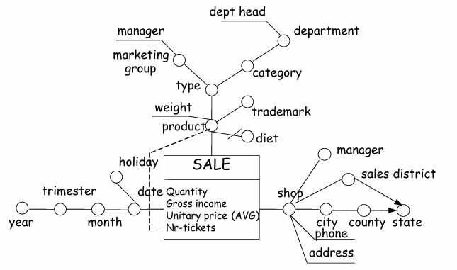
The fact schema would be created by defining “Sale” as the primary fact, with dimensions like “Time,” “Location,” and “Product” set up as hierarchies that enable analysis across different levels of aggregation. Measures such as “Quantity Sold” and “Total Revenue” provide quantitative insights, while the dimensions allow users to explore these measures across various contexts, such as by time period or geographic region.