Data Preprocessing for ML Fraud Detection Systems

In practice, while the idea is that “the bigger the better” for data, the reality is that real data is often “dirty”. This means that it is riddled with inconsistencies, incompleteness, duplication, and other issues that render the data unusable and the results unreliable. It is crucial to apply data filtering mechanisms to clean and reduce the data. Even the smallest error can render the data completely unusable and invalidate the results.

There are a variety of different sources that provide different types of information:

• Transactional data refers to structured and detailed information that captures the important attributes of customer transactions. This data can be summarized over longer time periods by aggregating it. Summarization techniques such as calculating averages, identifying trends, determining maximum or minimum values, and analyzing recency, frequency, and monetary aspects can provide valuable insights for fraud detection and anti-money laundering purposes. The individual interpretation of transactional data and its interaction with other factors can be highly beneficial in identifying suspicious activities.
• Contractual, subscription, or account data
• Sociodemographic information
• Surveys
• Behavioral information
• Unstructured data
• Contextual or network information
• Qualitative, expert-based data
• Publicly available data, … and many more

To perform descriptive and predictive analytics, it is necessary to have structured data that can be easily processed and analyzed.

Definition

A structured data table consists of rows representing entities (such as customers, transactions, enterprises, claims, cases) and columns containing information about these entities.

To create an aggregated, non-normalized data table, multiple normalized source data tables need to be merged. This involves selecting relevant information from different tables and copying it into the aggregated table. The key attribute is used to identify and relate observations from different source tables belonging to the same entity. It is important to carefully manage the merging process to ensure accurate integration of all information.

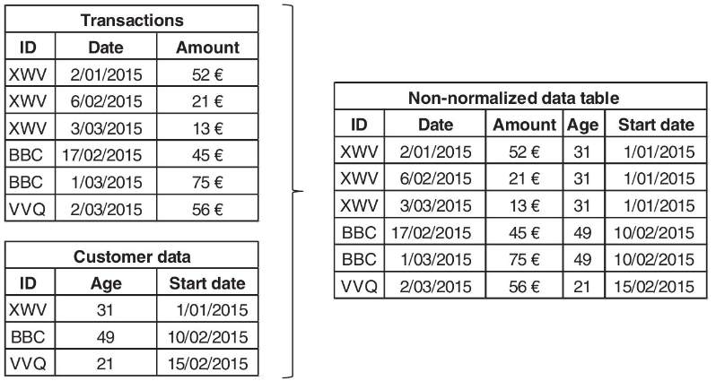
There are different types of data elements that can be encountered in datasets:

1. Continuous data: These are data elements that are defined on an interval and can have both limited and unlimited values. Continuous data can include measurements such as temperature, time, or weight, where there is a range of possible values.
2. Categorical data: Categorical data refers to data elements that fall into distinct categories or groups. There are three subtypes of categorical data:
   • Nominal data: This type of data consists of elements that can only take on a limited set of values with no meaningful ordering in between. Examples of nominal data include colors, genders, or categories of products.
   • Ordinal data: Ordinal data is similar to nominal data in that it also consists of elements with a limited set of values. However, in ordinal data, there is a meaningful ordering or hierarchy between the values. For example, a survey response scale ranging from “strongly disagree” to “strongly agree” represents ordinal data.
   • Binary data: Binary data is a special case of categorical data where the elements can only take two values, typically represented as “yes” or “no,” “true” or “false,” or “1” or “0.” Binary data is commonly used to represent yes/no questions or the presence/absence of a certain characteristic.

Sampling

Definition

Sampling is the process of selecting a subset of observations from a larger population to estimate characteristics of the population. Sampling is used in many areas of data analysis, including fraud detection, to reduce the computational burden and improve the efficiency of the analysis.

Take a subset of historical data to construct an analytical model. Despite the availability of high-performance computing, analyzing the entire dataset directly may not be necessary. It is important to ensure that the sample is representative of future entities and to choose the optimal time window. Timing and representativeness are critical factors.

Sampling timing and bias: There is a trade-off between having a large amount of data for a more robust analytical model and using recent data for better representativeness. It is ideal to select an “average” period that provides an accurate depiction of the target population. It is important to avoid sampling bias, even though it may not be a straightforward task.

Example in the context of credit cards

When analyzing a month’s worth of data, it is important to consider which month is representative. For instance, during the month of December, customers may use their credit cards differently due to holiday shopping. This can introduce two sources of bias compared to normal business periods.

1. Firstly, credit card customers may spend more during this period, both in total and on individual products.
2. Secondly, they may purchase different types of products from stores they don’t typically frequent.

There are various ways to mitigate the seasonality effect or bias:

1. One approach is to create separate models for different months or homogeneous time frames. However, this solution is complex and resource-intensive, as it requires developing, running, maintaining, and monitoring multiple models.
2. Another option is to sample observations over a period that covers a full business cycle and build a single model. This approach may result in reduced fraud detection power, as the model is less tailored to a specific time frame. However, it is a less complex and costly solution to implement.

The choice of sampling method directly impacts the effectiveness of fraud detection: by selecting a representative sample, the model can be more accurate and reliable, but it may also be more complex and resource-intensive.

In the context of fraud detection, stratified sampling is a technique used to create a sample that reflects the distribution of the original data. This is particularly important when dealing with highly skewed datasets. There are two main approaches to stratified sampling in fraud detection:

1. Stratifying based on the target fraud indicator: This involves creating a sample that maintains the same proportion of fraudulent and non-fraudulent transactions as the original data. This ensures that the sample accurately represents the fraud patterns in the dataset.
2. Stratifying based on predictor variables: This approach aims to create a sample that resembles the distribution of real product transactions. By stratifying the sample based on relevant predictor variables, such as transaction type or customer demographics, the resulting sample will better capture the characteristics of the original data.

Using stratified sampling techniques in fraud detection helps ensure that the sample accurately represents the underlying patterns and distributions in the data, improving the effectiveness of subsequent analysis and modeling.

Visual Data Exploration

Initial insights into the data can be gained by visualizing it using various plots and graphs. These visual representations help in understanding the distribution and patterns present in the data. Here are some commonly used plots and graphs:

1. Pie chart: A pie chart is a circular chart divided into sectors, where each sector represents a category or proportion of the whole. It is useful for displaying the relative proportions of different categories in the data.
2. Bar charts: Bar charts use rectangular bars to represent data. They are commonly used to compare and display categorical data. The length of each bar represents the frequency or value of the category it represents.
3. Histogram: A histogram is a graphical representation of the distribution of numerical data. It consists of a series of bars, where the height of each bar represents the frequency or count of data falling within a specific range or bin.
4. Scatter plots: Scatter plots are used to visualize the relationship between two numerical variables. Each data point is represented by a dot on the plot, with the x-axis representing one variable and the y-axis representing the other. Scatter plots are useful for identifying patterns, trends, and correlations in the data.

Exploratory Statistical Analysis

To gain insights and identify any differences between fraudsters and non-fraudsters, it is important to perform exploratory statistical analysis. This involves using descriptive statistics to provide basic measurements and information about the data.

Descriptive statistics can include measures such as the mode (most frequently occurring value for categorical variables), the mean or standard deviation (indicating the spread of the data around the mean), and percentiles (complementing the distribution and identifying the median value). These measures help provide a comprehensive understanding of the data. In addition to descriptive statistics, visual inspection of the distributions of the variables can also be helpful. This includes assessing aspects such as skewness, peakedness, or flatness of the distribution. Visual plots can provide a clearer understanding of these aspects.

It’s important to note that while descriptive statistics and visual inspection are valuable tools, they have limitations and may not always provide a complete picture. In some cases, alternative techniques like Benford’s Laws may be used to assess the symmetry or asymmetry of a distribution.

Dealing with Missing Values

Missing values can occur for various reasons, such as non-applicable information, undisclosed data, or errors during data merging. When working with missing values, different techniques can be employed:

1. Replace: Replace the missing value with a known value. This can be done using methods like mean imputation or regression imputation.
2. Delete: Delete observations or variables with a large number of missing values. This assumes that the missing values are random and have no meaningful relationship with the target variable.
3. Keep: Sometimes, missing values can be meaningful and may have a relationship with the target variable, such as in the case of fraud. In such cases, the missing values can be treated as a separate category.

To determine the appropriate approach, it is important to statistically test whether the missing information is related to the target variable. If there is a relationship, the “keep” strategy can be adopted by creating a special category for the missing values. If there is no relationship, the decision to delete or replace missing values can be based on the number of available observations.

ID	Age	Income	Marital Status	Credit Bureau Score	Fraud
1	34	1,800		620	Yes
2	28	1,200	Single		No
3	22	1,000	Single		No
4	60	2,200	Widowed	700	Yes
5	58	2,000	Married		No
6	44				No
7	22	1,200	Single		No
8	26	1,500	Married	350	No
9	34		Single		Yes
10	50	2,100	Divorced		No

Outliers

Definition

An outlier is an observation that is significantly different from other observations in the dataset. Outliers can be valid or invalid, and they can have a significant impact on the results of data analysis.

They are categorized into two main types: valid and invalid outliers.

1. Valid Outliers: These are extreme but plausible values within the dataset. For example, a high executive salary of $1,000,000 might be a valid outlier in a dataset of employee salaries. Although it is significantly higher than the average, it is a legitimate value that reflects a real-world scenario.
2. Invalid Outliers: These observations are erroneous or unrealistic. For instance, an age of 300 years is clearly not feasible and indicates an error in data recording or entry.

Outliers can also be classified based on the dimensionality of their extremeness:

• Univariate Outliers: These outliers are extreme in a single variable or dimension. For example, if you are analyzing the height of individuals and one data point is 8 feet tall, this would be considered a univariate outlier. The assessment of such outliers can be performed by setting minimum and maximum threshold values for the variable in question.
• Multivariate Outliers: These outliers are extreme across multiple variables simultaneously. For instance, if a data point has an extremely high value for both salary and years of experience compared to other data points, it might be considered a multivariate outlier. Identifying multivariate outliers often involves more complex statistical techniques such as Mahalanobis distance or principal component analysis.

To identify and manage outliers, various methods and tools can be employed:

1. Graphical Tools:
   • Histograms: Useful for visualizing the distribution of a single variable and spotting extreme values.
   • Box Plots: These display the distribution of data based on quartiles. They show the median, first quartile (Q1), third quartile (Q3), and potential outliers. Outliers are typically represented as points that lie outside the range defined by 1.5 times the interquartile range (IQR) from the quartiles.
2. Statistical Measures:
   • Z-Scores: This method involves calculating the number of standard deviations an observation is from the mean of the dataset. The formula for the Z-score of a data point () is: where () is the value of the observation, () is the mean of the dataset, and () is the standard deviation. A Z-score beyond or is often considered indicative of an outlier.

ID	Age	z-Score
1	30
2	50
3	10
4	40
5	60
6	80
…

In the case of multivariate outliers, one approach is to fit regression lines and examine the observations with large errors, such as through a residual plot. Another method is to use clustering or calculate the Mahalanobis distance.

When it comes to outlier detection and treatment, there are various strategies available:

• For invalid observations, treating the outlier as a missing value is a common approach.
• For valid observations, it is possible to impose both a lower and upper limit on a variable, bringing any values below or above these limits back to the limits.

An example of truncation is when both a lower and upper limit are imposed on a variable, and any values below or above are adjusted to match these limits.

Other techniques for outlier detection and treatment include using Z-scores, applying a sigmoid transformation that ranges between and using the function .

Expert-based Outlier Detection

In expert-based outlier detection, domain-specific knowledge is leveraged to create a set of rules or criteria that guide the identification of potential anomalies in the data. These rules are crafted by subject matter experts who understand the intricacies of the data, the relationships between variables, and the expected behavior under normal conditions. This approach ensures that the detection process is tailored to the specific context of the data, leading to more accurate and meaningful results. To effectively apply expert-based outlier detection, rules must be systematically formulated. These rules can be designed to address various aspects of the data, including:

1. Inter-variable Relationships: Experts can define rules that consider the relationships between different variables in the dataset. For example, if variable is typically higher when variable is lower, a rule can be established to flag instances where this relationship does not hold. Such relationships are often complex and context-dependent, making expert input crucial.
2. Variable Value Constraints: Constraints can be defined for specific combinations of variable values. For instance, in a dataset containing patient health records, a rule might stipulate that certain combinations of symptoms are highly unlikely or impossible. If these combinations appear, the rule would flag them as potential outliers. These constraints help to catch subtle errors or inconsistencies that might otherwise be missed by standard statistical methods.

Expert-based outlier detection offers several advantages over purely algorithmic methods:

• Context Awareness: Rules derived from expert knowledge are inherently context-aware, making them more likely to identify relevant outliers that are meaningful within the specific domain.
• Flexibility: Experts can adapt the rules over time as new insights are gained or as the underlying data changes. This flexibility ensures that the outlier detection process remains effective even as conditions evolve.
• Targeted Detection: By focusing on specific relationships and constraints, expert-based rules can target particular types of anomalies that may be of greater concern, rather than flagging large numbers of irrelevant data points.

The scope of expert-based outlier detection is broad and can be applied across various fields such as healthcare, finance, manufacturing, and more. In healthcare, for instance, expert-based rules can be used to detect unusual combinations of diagnostic codes or unexpected lab results. In finance, these rules might flag transactions that deviate from expected patterns based on historical data. The technical complexity lies in the formulation and continuous refinement of these rules, ensuring they remain aligned with both the data’s evolving nature and the domain’s requirements.

Example

When analyzing customer data, if a customer’s birth date is listed as “01/01/1980” and their category is listed as “child,” it is difficult to determine which value is invalid. Neither value is considered an outlier, so an analyst may not notice this conflicting information unless specific precautions are taken.

Discussion on preprocessing

When working with valid outliers in the dataset, it is important to be cautious about the treatment techniques used, especially when applying unsupervised learning techniques for fraud detection. Treating valid outliers in a way that impairs the ability of unsupervised learning algorithms to detect fraud can have negative consequences.

On the other hand, when dealing with invalid outliers, it is recommended to treat them as missing values. This can be done by including an indicator that the value was missing or, for more accuracy, identifying it as an invalid outlier.

Euclidean vs Manhattan

The Euclidean distance is the straight-line distance between two points in a Euclidean space. It is the most common distance metric used in machine learning and data analysis. The formula for calculating the Euclidean distance between two points and is:

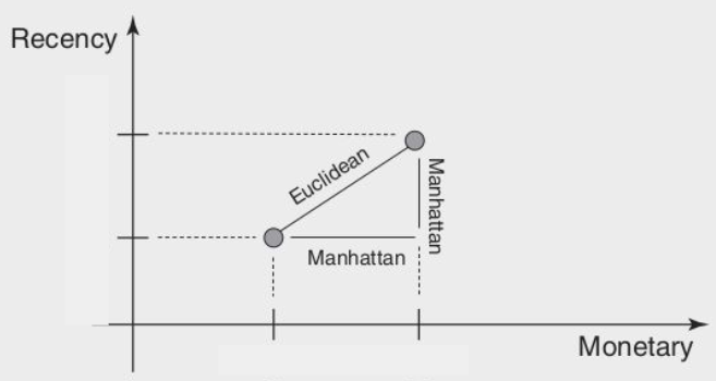
The Manhattan distance, also known as the taxicab distance, is the sum of the absolute differences between the coordinates of two points. The formula for calculating the Manhattan distance between two points and is:

Data Standardization

Data standardization is a crucial preprocessing step in data analysis and machine learning, ensuring that all variables are on a comparable scale. This process mitigates the influence of variables that may otherwise dominate due to differences in units or magnitudes. Here are some common methods of data standardization:

• Min/Max Standardization: This technique rescales the data so that the values fall within a specified range, typically between and . The formula used is: where () is the original value, and () and () are the minimum and maximum values in the dataset, respectively. Min/Max standardization is particularly useful when the features have different units or scales but you want them to contribute equally to the analysis.
• Z-score Standardization: This method transforms the data to have a mean of and a standard deviation of . It is accomplished by calculating the z-scores for each data point: where () is the original value, () is the mean of the dataset, and () is the standard deviation. Z-score standardization is beneficial when the data follows a normal distribution, making it suitable for algorithms that assume normally distributed data.
• Decimal Scaling: In this approach, the data is scaled by dividing each value by a power of . The power is determined by the maximum absolute value of the dataset, ensuring the data falls within a manageable range. This method is simple and effective, especially when dealing with datasets with varying scales that need to be normalized without altering the data structure significantly.

Categorization of Variables

When working with categorical variables or continuous variables that need to be discretized, it’s often necessary to reduce the number of categories or to group continuous values into bins. This process simplifies the data, making it more manageable and often more interpretable.

• Equal Interval Binning: This method divides the range of continuous variables into equal-sized intervals, assigning each data point to a bin based on its value. It is particularly useful when the data is uniformly distributed, as it ensures that each bin has a comparable range of values.
• Equal Frequency Binning: Unlike equal interval binning, equal frequency binning creates bins that contain an approximately equal number of observations. This method is advantageous when the data is skewed, as it ensures that each bin has a similar representation of data points, making it easier to compare categories.
• Chi-Squared Analysis: This statistical technique assesses the relationship between categorical variables by calculating the chi-squared statistic. It helps in determining whether the observed frequencies of categories differ significantly from the expected frequencies. Chi-squared analysis is particularly useful for identifying and merging similar categories, thereby reducing the number of levels in a variable while retaining its predictive power.
• Pivot Table: A pivot table is an aggregation tool that allows for summarization and exploration of data based on different categorical variables. It provides a clear overview of how different variables interact and is essential for initial data exploration, especially when dealing with large and complex datasets.

For continuous variables, categorization can be applied to address non-monotonic relationships with the target variable by grouping the continuous data into meaningful ranges. This approach can reveal patterns that might be obscured in the raw data, leading to more robust model performance.

Variable Selection

In analytical modeling, particularly in fields such as fraud detection, it’s common to start with a large number of variables, many of which may not contribute significantly to the prediction of the target variable. Effective variable selection is crucial to build more efficient and accurate models.

• Filters: Filters are a quick and straightforward method for selecting relevant variables. They evaluate each variable’s individual correlation with the target variable, allowing for an early reduction in the number of variables. This method is efficient for handling high-dimensional data, but it only considers univariate correlations, meaning it does not account for the relationships between variables. As a result, some important variables may be overlooked, or redundant variables may be retained.

• Principal Component Analysis (PCA): PCA is a dimensionality reduction technique that transforms the original variables into a new set of uncorrelated variables called principal components. These components capture the maximum variance in the data. PCA reduces the number of dimensions by focusing on the components that explain the most variance, thus simplifying the dataset. However, while PCA is powerful in reducing dimensionality, it also reduces interpretability, as the principal components are linear combinations of the original variables. This trade-off between dimensionality reduction and interpretability must be carefully considered, especially in contexts where understanding the contribution of each variable is important.

  PCA is especially useful when dealing with datasets that have multicollinearity, as it helps in eliminating redundancy by focusing on the independent components. However, the reduction in interpretability might not be suitable for all applications, particularly those requiring clear explanations of model decisions, such as in regulatory environments.

Additional Considerations

While standardization, categorization, and variable selection are essential steps in data preprocessing, it is also important to consider additional factors that may influence these processes. For example, in certain industries, variables may need to be selected or standardized based on privacy regulations or operational constraints. Understanding the broader context in which data is used ensures that the preprocessing steps align with both technical requirements and business needs, leading to models that are not only accurate but also compliant and practical for deployment.