Definition
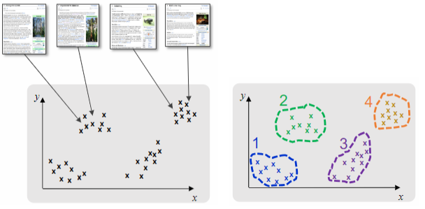
Clustering is the process of grouping documents based on some distance function or similarity measure into coherent subgroups.
For text documents, usually we group documents into clusters based on:
- the same topic: sports, politics, etc.
- same emotions: positive, negative, etc.
- same problem or task to be fixed: no heating in office, unable to print, etc.
- same complaint or praise: good service, bad service, etc.
- same author
- same text generator
- same original source document
On the Google News website, text grouping is employed to summarize and categorize news articles. The clustering process takes into account factors such as topics, relevance, and trends to provide a comprehensive overview of the collection. This approach allows users to easily navigate and access the most relevant and trending news articles based on their interests.
In security applications, such as detecting phishing and malware, it is often necessary to identify potentially malicious groups based on a few known instances. Clustering is used in this scenario to uncover relevant document features, which can then be used to classify new documents. This approach helps in the classification and detection of security threats, enabling proactive measures to be taken against potential attacks.
Document Representation and Similarity
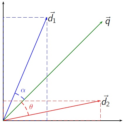
To perform document clustering, it is essential to assess the similarity between documents, which is subjective and varies depending on the specific application. Typically, documents are represented as TF-IDF vectors, which capture the importance of words in the document. This representation is sparse, with many zero values. Therefore, a common approach is to measure similarity based on the shared words, taking into account their importance. By considering the number of shared words and their relevance, we can effectively determine the similarity between documents and cluster them accordingly.
Usually, we assume that the similarity doesn’t depend on the length of the documents, so we compute cosine similarity between vectors; this is the same to compute the dot-product between the length-normalised vectors.
where
Clustering techniques
There are many clustering algorithms that can be used to group text documents. Some of the most common are:
- k-means and k-medoids
- Hierarchical-agglomerative clustering
- Density-based clustering (DBSCAN)
- Spectral clustering
- Topic models (LDA, LSA)
All these models are implemented in the scikit-learn library, which is a powerful tool for text clustering.
K-means
Definition
k-means is a clustering algorithm that partitions data into
clusters by minimizing the within-cluster sum of squares.
This algorithm searches for exactly
Definition
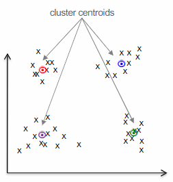
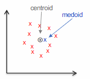
A centroid is the point that minimizes the sum of squared distances to all other points in the cluster. In other words, it is the average of all the points in the cluster.
The key benefits of using
Additionally, the number of clusters must be predetermined before running the algorithm.
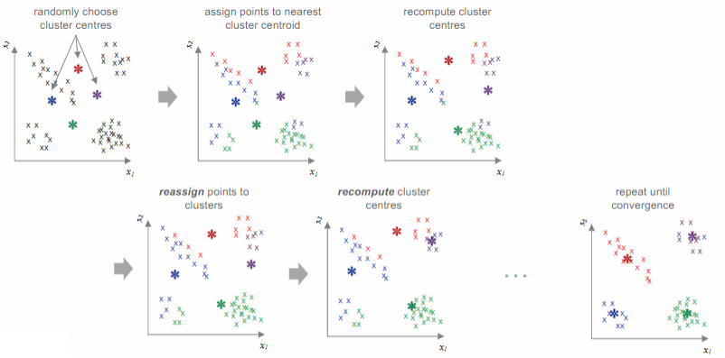
The k-means algorithm
Initialize
centroids randomly (re)assign each data point to the closest centroid using the formula:
(re)compute the centroids by averaging the data points in cluster
repeat steps 2 and 3 until convergence, when the centroids stop moving
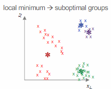
Potential challenges with
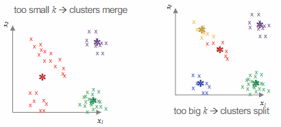
Another concern is the possibility of the algorithm converging on a local minimum, so it is advisable to run the algorithm multiple times with different initializations.
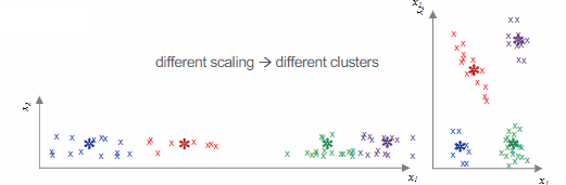
Similar to other clustering algorithms, scaling can impact the similarity measure and consequently the clusters obtained. However, for text data, the utilization of TF-IDF weighting and document length normalization mitigates the scaling issue.
K-medoids
The k-medoids algorithm is a clustering technique that, unlike
Definition
The medoid is one of the data points in the datasets, and it’s the point that is the closest (smallest average distance) to all the other points in the cluster.
Unlike the centroid (which is a theoretical point often calculated as the mean of all points in the cluster and may not correspond to an actual data point), the medoid is one of the actual data points in the cluster. It is defined as the point with the smallest average distance to all other points in the cluster. In other words, the medoid is the most centrally located point within the cluster, minimizing the sum of distances to other points.
The k-medoid algorithm
The
-medoids algorithm follows an iterative process similar to -means but with key differences due to the use of medoids:
- Initialization: The algorithm starts by selecting
initial medoids randomly from the dataset. - Assignment Step: Each data point in the dataset is assigned to the cluster whose medoid is the closest, based on a chosen distance metric (such as Euclidean, Manhattan, or others).
- Update Step: For each cluster, the algorithm then searches for a new medoid by evaluating each point in the cluster to determine if it would serve as a better medoid — i.e., if it would reduce the total sum of distances to all other points in the cluster.
- Iteration: Steps 2 and 3 are repeated until the medoids stabilize and no longer change between iterations, indicating that the optimal clustering has been found.
The
However, the
Hierarchical Agglomerative Clustering
The process of hierarchical clustering involves constructing a dendrogram, which represents a hierarchy of clusters. In the agglomerative approach, clusters are formed by merging groups of documents from the bottom-up. This means that the algorithm follows these steps:
- Initially, each document is assigned to its own individual group.
- The two groups that are most similar are merged together.
- Steps 2 is repeated until only one group remains.
graph TB
	a ---> abcdef
	b --> bc --> bcdef --> abcdef
	c --> bc
	d --> de --> def --> bcdef
	e --> de
	f --> def
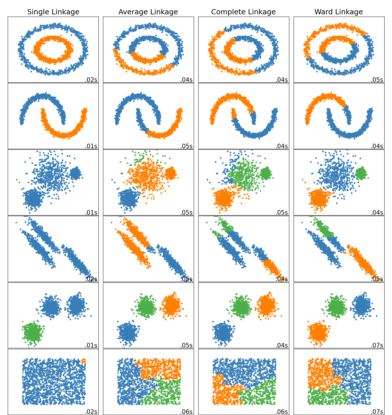
To determine the distance between groups, a linkage criteria can be applied. The commonly used linkage criteria include:
- Single linkage: calculates the minimum distance between any two points in the two groups.
- Complete linkage: measures the maximum distance between any two points in the two groups.
- Average linkage: computes the average distance between all pairs of points in the two groups.
NOTE
The linking criteria used influences the shape of the clusters found. Complete or average linkage will restrict to tight, globular clusters, while single linkage will allow for finding long and thin clusters.
The main advantage of hierarchical clustering is that it works with any distance metric or similarity function, and the dendrogram representation provides information about the underlying structure of the data. However, the algorithm is computationally expensive, making it impractical for large datasets.
DBScan
DBScan, short for Density-Based Spatial Clustering of Applications with Noise, is an algorithm that determines the number of clusters based on the data itself. It identifies clusters as regions of high density separated by regions of low density. The algorithm relies on two parameters:
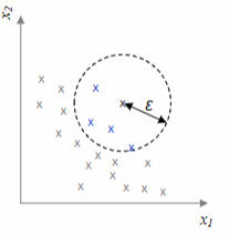
The algorithm works as follows: the number of datapoints in the
- Core point: if the number of points in the
-neighborhood is greater than - Border point: not core, but in the
-neighborhood of a core point - Noise point: neither core nor border
The benefits of DBSCAN include its ability to automatically determine the number of clusters, its ability to identify and disregard noise points, and its capability to detect clusters of various shapes. However, the performance of DBSCAN heavily relies on the selection of the parameters
Evaluating clustering
Assessing the quality of a clustering is not an easy task, because usually we don’t have access to ground-truth labelling. Without it, evaluation can be subjective (people might disagree on what “right” clusters are). There are two ways to evaluate the results of a clustering algorithm:
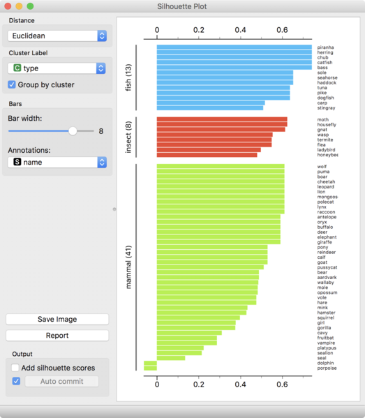
- Intrinsic evaluation: This evaluation assesses the coherence and separation of clusters. It typically measures the within-cluster sum of squares (cluster variance) and the silhouette coefficient (compares the average distance to points in the current cluster with points in the next closest cluster).
- Extrinsic evaluation: This evaluation examines how well the clusters align with known document labels. It measures homogeneity (how well each cluster contains only members of a single class), completeness (how well all members of a given class are assigned to the same cluster), and the V-measure (the harmonic mean of homogeneity and completeness).
Intrinsic evaluation measures can be helpful in visualizing the quality of clusters through Silhouette plots. To select a value for
If ground-truth labels knows various metrics can be used to evaluate clustering performance. We can evaluate the clustering output as classification prediction, by assigning the majority class to each cluster, compute the Precision, Recall and F1-score for each class, and then compute the average of these metrics. Alternatively, we can use the measures designed for clustering, like:
- Homogeneity (
): reduction in uncertainty of class given the clusters - Completeness (
): reduction in uncertainty of cluster given the classes - V-measure (
): harmonic mean of homogeneity and completeness - Uncertainty measured using entropy for cluster assignments
Elbow method
The Elbow method is a technique used to determine the optimal number of clusters in a dataset. It involves plotting the within-cluster sum of squares (WCSS) against the number of clusters. The WCSS is calculated as the sum of the squared distances between each data point and the centroid of the cluster to which it belongs.
The Elbow method helps identify the point at which the rate of decrease in WCSS slows down, indicating the optimal number of clusters. The “elbow” point is the optimal number of clusters, as it represents the point at which adding more clusters does not significantly reduce the WCSS.
Silhouette coefficient
The Silhouette coefficient is a measure used to assess the quality of clustering. It calculates a score for each sample individually, using a distance metric such as Euclidean distance. The coefficient is computed by finding the average distance from a sample
Silhouette plots are often used to visualize the quality of clusters. However, calculating the Silhouette coefficient can be computationally expensive as it needs to be done independently for each datapoint.
Sum of Squares
It is very common to compute the sum of squares values in clustering analysis. This includes:
- The within-cluster sum of squares (WSS) is a metric that calculates the squared distances between the centroid of a cluster and each point within that cluster. It provides a measure of how tightly the data points are clustered around the centroid.
- The between-cluster sum of squares (BSS) is a metric that calculates the squared distances between the centroid of the data and each cluster centroid, taking into account the weights of the data points.
- Variance Ratio Criterion (or Calinski-Harabasz index), combines both measures into a single metric. This index assesses whether clusters are dense and well separated. It is faster to compute than the Silhouette index, but ultimately serves as an objective function for the k-Means algorithm.
Topic modelling
Definition
Topic modelling is a soft clustering of documents allowing documents to belong to multiple clusters.
It offers a reduced-dimensional representation of documents compared to the high-dimensional vocabulary space. Each cluster is known as a “topic” and is characterized by a distribution of words. The terms within a topic should be coherent, indicating that they pertain to the same subject. The topic vector represents the probability distribution of words in the vocabulary, while the document vector represents the probability distribution of topics.
Topic modelling is a form of matrix decomposition, that decomposes the
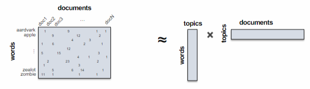
The renowned algorithm for topic modelling is called Latent Dirichlet Allocation (LDA). It derives its name from the utilization of a Dirichlet prior during parameter estimation. LDA is closely related to other techniques such as Non-negative Matrix Factorization (NMF), as well as Latent Semantic Indexing (LSI) which employs Singular Value Decomposition (SVD) on the term-document matrix.
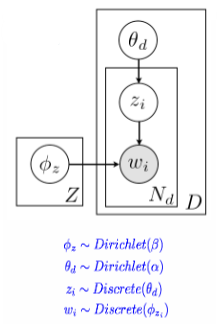
Latent Dirichlet Allocation (LDA)
The LDA generative model for latent Dirichlet allocation involves several steps.
- First, word proportions for each topic are chosen.
- Then, topic proportions for each document are chosen.
- For each position in the document, a topic is chosen based on the document proportions, and a word is chosen based on the topic proportions.
Estimating parameters for the topic model requires iterative updates of parameters, topic probabilities for each document, and word probabilities for each topic. Bayesian priors are placed on the parameters to prevent overfitting, and Gibbs sampling is used to avoid local maxima. The hyperparameters
and determine the prior on the topic/document distributions.
Factorization and clustering techniques enhance the representation of documents by generalizing the observed term counts. This results in denser and more meaningful document representations, enabling the calculation of more relevant distances between documents.
Topic modeling addresses challenges such as polysemy (words with multiple meanings), synonymy (multiple words with the same meaning), and short documents with limited vocabulary. It can be valuable for visualizing collections by further reducing dimensionality and representing topics based on the most frequent terms. Additionally, topic modeling is commonly used to track the evolution of topics over time in collections.
Dimensionality reduction techniques
Can project high-dimensional data into lower dimension using:
- a linear projection with PCA (Principal Component Analysis)
- a non-linear projection using t-distributed Stochastic Neighbor Embedding (t-SNE)
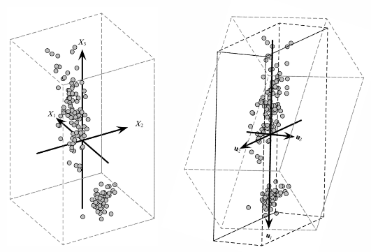
PCA (Principal Component Analysis)
Principal Component Analysis investigates the main sources of variation in dataset by finding the projection that carputers the largest amount of variation in data.
The PCA algorithm
- Scale the features to have zero mean and unit variance.
- Find the direction in the original high-dimensional space that represents the largest variation in the data (choose a lower-dimensional space with fewer dimensions, denoted as
). - Remove the variation captured by the chosen direction from the data.
- Repeat steps 2 and 3 until
dimensions are found. The new lower-dimensional space can be used to approximate the original data by considering only the largest components.
t-SNE (t-distributed Stochastic Neighbor Embedding)
Data in high dimensions do not occupy the entire space, but rather reside on lower-dimensional manifolds.
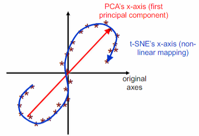
The t-SNE algorithm is a non-linear method for reducing the dimensionality of data. It is commonly used to map high-dimensional data onto a 2D or 3D space. Unlike PCA, t-SNE creates a non-linear combination of the original attribute values to represent the mapped points. The axes in the mapped space are obtained through a non-linear transformation (rotation) of the original axes.
t-SNE is a dimensionality reduction algorithm that focuses on preserving the local distances between nearby points, unlike PCA which aims to preserve the global distances between all points. It achieves this by converting distances between data points into joint probabilities and then mapping the original points to lower-dimensional points. The position of the mapped points is chosen in a way that preserves the underlying structure of the data, ensuring that similar data points are assigned to nearby map points and dissimilar data points are assigned to distant map points.
The t-SNE algorithm
The t-SNE algorithm consists of two main steps:
- Defining a probability distribution over pairs of high-dimensional points, where similar data points have a high probability of being chosen and dissimilar points have an extremely low probability.
- Defining a similar distribution over the points in the map space and adjusting the positions of the mapped points to minimize the Kullback-Leibler divergence between the two distributions. This is achieved through the use of gradient descent to iteratively minimize the score.
Caveats of t-SNE include the perplexity parameter, which determines the trade-off between local and global aspects of the data. Different initializations can result in different outcomes. Additionally, t-SNE is suitable for data with a moderate number of dimensions (around 30-50), as computational time becomes a limiting factor for higher-dimensional data.