7 - Static Flow Analysis of Programs

---

Static flow analysis is a critical technique used in compiler design to transform high-level source code into efficient machine code. This process involves multiple stages, each with distinct objectives and methodologies. During the first stage of compilation, the source program is converted into an intermediate representation. This intermediate form acts as a bridge between high-level programming languages and machine language, providing a format that is closer to the machine’s operational domain while retaining enough abstraction to facilitate further analysis and optimization.

In the subsequent stage, static flow analysis is applied to this intermediate form. This stage serves multiple purposes. Verification is one key goal, focusing on rigorously ensuring the correctness of the program. It involves sophisticated checks to detect logical errors or inconsistencies that might have been missed during earlier syntactical analyses. Another significant aim is optimization, where transformations are made to improve the program’s execution efficiency. This can involve tasks such as register allocation, which optimizes the use of the processor’s registers to minimize memory access overhead. Additionally, instruction scheduling is performed, which reorganizes the sequence of instructions to enhance pipeline utilization and overall performance, ensuring a smooth and efficient execution flow on modern hardware architectures.

A useful abstraction in static flow analysis is the control flow graph (CFG), which models the program as an automaton. This automaton represents a specific program rather than the entire programming language, emphasizing the distinction between static flow analysis and syntax-driven translation. The automaton is particularly useful for analyzing the program’s behavior, as it captures the sequence of operations that the program can execute—referred to as its execution trace. Through the lens of automata theory, the execution trace is treated as a string recognized by the automaton, enabling the application of formal methods to study program properties.

The methods employed in static flow analysis draw heavily from automata theory, formal logic, and statistics. For the purposes of this discussion, automata theory is of primary interest. Here, the program is treated as a simplified automaton, where only the most fundamental instructions in the intermediate form are considered. These include scalar variables, constants, assignments, and basic unary arithmetic, logic, or relational operations. The analysis is further restricted to intraprocedural analysis, meaning it focuses on the flow within a single procedure or function, rather than considering interprocedural interactions across the entire program.

Program Control Graph (PCG)

The Program Control Graph (PCG) is a structured representation used in static flow analysis to model the flow of control within a program. It provides a graphical abstraction where the nodes and edges correspond to program instructions and their execution order.

Key Features of the Program Control Graph:

1. Nodes Represent Instructions: Each node in the graph corresponds to a specific instruction or statement in the program.
2. Edges Indicate Execution Flow: If an instruction is immediately followed by another instruction during execution, there is a directed edge from to . Here, is the predecessor of .
3. Input and Output Nodes:
   • The initial node (input node) represents the first instruction of the program.
   • The final node (output node) represents an instruction without successors, marking the program’s end.
4. Conditional Instructions: Nodes corresponding to conditional statements have multiple outgoing edges, each representing a possible execution path.
5. Confluence Nodes: An instruction with two or more incoming edges is a confluence node (or merge/join node), representing a point where multiple execution paths converge.

Despite its utility, the PCG has certain limitations. For example, it does not represent the logical values of conditions (true/false) that determine the successor of a conditional instruction. Additionally, assignment operations are abstracted to capture the relationships between variables, distinguishing between variable definitions and uses.

Variable Analysis in the PCG

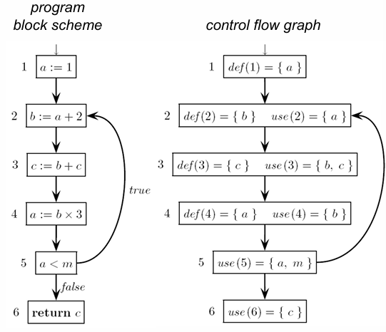
Each node in the PCG is associated with two sets:

• : The set of variables defined (assigned a value) by the instruction at .
• : The set of variables used (read) by the instruction at .

Examples:

1. Instruction:
   • : The variable is defined because it is updated.
   • : The variables and are used in the computation.
2. Instruction:
   • : The variable is defined.
   • : No variables are read.

It is noteworthy that two instructions with the same and sets are indistinguishable in the control flow graph.

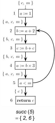
Example Program and Its Control Flow Graph

Consider the following example program:

     a := 1
e_1: b := a + 2
     c := b + c
     a := b * 3
     if a < m goto e_1
     return c

This program can be represented as a control flow graph where nodes are labeled with instructions, and edges represent the program’s control flow. For instance, instruction leads to a conditional , creating a branching structure.

Language of the Control Graph

Definition

The control flow graph corresponds to a finite-state automaton where:

• The alphabet consists of the instruction labels.
• Each node is represented as a triple , where and are the sets associated with the instruction.

The language recognized by this automaton contains all strings over that label paths from the initial state to a final state. Each string represents a sequence of instructions the program can execute.

Example

For example, in the program above:

• is the instruction set
• A valid path is , which translates to the string .
• The set of all possible paths forms a regular expression: .

The language of the control flow graph is local, belonging to a subset of the regular languages. Each node in the automaton has a unique label, ensuring that the paths through the graph can be uniquely identified. This property makes the control graph particularly suitable for analyzing program behaviors and verifying their correctness using formal methods.

Precautionary Approximation in Control Flow Graphs

Control flow graphs (CFGs) provide a structural representation of programs, but they inherently rely on approximations that can introduce inaccuracies. These approximations arise because CFGs do not explicitly model the logical conditions of branching instructions. Consequently, they may represent paths through the program that are theoretically impossible to execute.

Example of Unexecutable Paths

Consider the conditional statement:

The CFG generated for this snippet contains two branches:

1. Path , representing the execution of when .
2. Path , representing the execution of when .

However, is always non-negative due to the properties of squaring, making the second path () unexecutable. The CFG includes this invalid path because it does not consider the semantics of the condition .

This issue illustrates a fundamental limitation:

CFGs do not model the logical evaluation of conditions and, therefore, cannot distinguish between executable and unexecutable paths.

Determining whether a path in the CFG is executable is generally undecidable, as this problem is reducible to the Turing halting problem. The inability to decide executability stems from the complexity of program semantics, especially when the conditions involve arbitrary computations or external inputs.

Precautionary Diagnosis and Error Detection

The static flow analysis method involves examining all paths from the input node to the output node in the CFG. While this exhaustive approach ensures that all real errors are identified (making the method error-safe), it can also lead to false positives:

• Nonexistent errors may be diagnosed because of unexecutable paths in the CFG.
• Unnecessary resources may be allocated based on the analysis of paths that cannot occur during actual program execution.

Despite these inefficiencies, the method is robust in detecting all actual errors within the program.

Hypothesis: Reduced Form of the Automaton

For static flow analysis to be effective, the CFG should be in a reduced form.

This means:

1. All nodes must be reachable: Every node in the CFG should be accessible from the input node. Unreachable nodes represent dead code, which is code that can never be executed.
2. All nodes must be defined: Every node should contribute meaningfully to the program’s logic. Nodes without a valid role indicate inefficiencies or redundant instructions.

If the CFG is not in a reduced form, the following problems may arise:

• Program Inefficiency: The presence of redundant instructions could lead to unnecessary computation, increasing resource usage and runtime.
• Dead Code: Instructions that are never executed represent wasted effort and potential maintenance overhead.
• Infinite Loops: Non-reduced CFGs might contain loops that prevent the program from terminating.

Liveness Interval of a Variable

The liveness interval of a variable is a key concept in program analysis, particularly in optimizing compilers. It describes the segment of a program where the value of a variable is relevant, i.e., it may influence computations. Understanding liveness is essential for resource allocation tasks such as register allocation in compiler design.

Definition

A variable is said to be live at a program point if there exists a path in the control flow graph (CFG) from to another point where:

1. The path from to does not encounter any instruction (where ) that redefines , i.e., .
2. The instruction at uses , i.e., .

Thus, the variable is live at all points along the path from to , collectively forming its liveness interval.

Informally, a variable is live at a point if there exists an instruction that could eventually be executed, starting from , which uses the variable’s value.

Key Properties:

• A variable is live at the output of a node if it is live on at least one outgoing arc.
• A variable is live at the input of a node if it is live on at least one incoming arc.

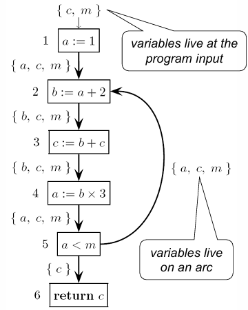
Example of Liveness

Let us consider the variable :

• is live at the input of node because there exists a path , where , and neither instruction nor defines .
• is live on paths and , but not on paths or .
• At the output of node , the variables are live.

Computing Liveness Intervals

To compute the liveness intervals for a variable, we analyze the control flow graph and use a formal definition of liveness conditions.

Definition

A variable is live at the output of a node if in the language of the automaton representing the CFG, there exists a sequence such that:

Here, is the set of instructions that define , and is the set of instructions that use .

The set of all strings satisfying the condition is a regular language:

To check if is live at the output of , we verify if is empty.

Computational Methods

• Recognizer-Based Method A recognizer for is constructed as the product of (the CFG automaton) and the recognizer for . Paths connecting the input node to any final node in the recognizer determine whether is non-empty. However, this approach is computationally expensive for large programs.

• Flow Equation Method This method is more efficient and simultaneously determines all live variables through a back-propagation computation scheme. The liveness sets are computed iteratively:

  1. For every final node :

  2. For every other node :

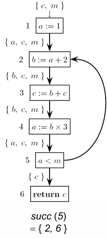
     Here, is the set of immediate successors of .

Example: Solving for Live Variables

Consider the following sets of instructions that define () and use () variables:

Variable

Step-by-step Solution:

1. Final Node :

2. Node :

3. Node :

4. Repeat this process for nodes to compute their liveness sets.

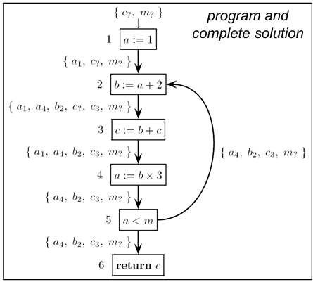
Solving Flow Equations Iteratively

Flow equations, commonly used in data-flow analysis, describe the relationships between program variables at different points in the control flow graph (CFG). Solving these equations provides insights into variable states, enabling optimizations such as dead code elimination, register allocation, or code motion. This process involves iteratively updating and refining approximations of variable sets until a stable solution is achieved.

Algorithm

In a program with nodes, the analysis requires solving equations corresponding to the input () and output () sets for each node . These sets represent whether variables are “live” (used or needed later) at a given point. Initially, the problem assumes no variables are live:

This initial approximation corresponds to the first iteration, . The algorithm then iteratively refines these sets by updating them according to the flow equations.

At each step , the algorithm computes new values for and by substituting the current values into the equations. The new solution is denoted as . If there is a change between consecutive iterations ( and ), the algorithm continues. If no changes occur, convergence is reached, and the solution is finalized.

Convergence is guaranteed after a finite number of iterations because:

1. The cardinality of and is bounded by the total number of variables in the program.
2. Each iteration either adds new variables to these sets or leaves them unchanged, ensuring monotonic growth.
3. Once no further updates are made, the algorithm terminates.

Example: Live Variable Analysis

Consider a program with six nodes, where the flow equations describe the relationship between and sets for each node. The equations are:

	in	out
1
2
3
4
5
6

The algorithm begins with all and sets empty. At each step, the sets are updated as follows:

Node	Iteration 0	Iteration 1	Iteration 2	Iteration 3	Final Solution
1
2
3
4
5
6

Technical Observations

1. Convergence: The analysis converges after four iterations, as no further changes occur to the and sets.

2. Monotonicity: At each step, the sets either grow or remain unchanged, ensuring the algorithm progresses towards termination.

3. Applications: This analysis helps identify variables needed at different points, enabling removal of unnecessary instructions, better memory management, and register allocation.

Final Results

At convergence, the liveness sets for each node are:

Node
		∅

These results give the final liveness intervals for the variables in the program.

Applications of Flow Equations Beyond Liveness Analysis

The flow equation method, used for analyzing liveness of variables, has broader applications in program optimization, such as memory allocation, identifying useless definitions, and reaching definition analysis. Let’s delve into each application with examples.

Memory Allocation

The liveness sets derived from flow equations help in determining which variables interfere with each other. Two variables interfere if their liveness sets overlap, meaning they are simultaneously live. This property is critical for register allocation or memory optimization.

Key Idea:

• Variables that do not interfere can share the same register or memory location.
• Interference is determined using sets of the nodes.

Example

From the previous analysis:

• Interfering pairs:
  • and (both in ),
  • and (both in ).
• Non-interfering pairs: (not simultaneously live in any set).
• Register allocation: For variables , three registers suffice because:
  • and can share a register.
  • and need separate registers due to interference.

Modern compilers use this principle with graph coloring algorithms to allocate variables efficiently.

Useless Definitions

Definition

A definition of a variable is useless if the variable is not live on any outgoing edge of the instruction.

Eliminating such instructions reduces program size and can expose further optimization opportunities.

Steps

1. For a given instruction defining variable , check whether .
2. If , the instruction is useless and can be eliminated.

Example

Using the previous liveness sets:

• Instruction 3 defines , but . Hence, instruction 3 is useless.
• Eliminating instruction 3:
  • The program becomes shorter.
  • Variable is removed from , , , and .
• Optimized flow equations enable further simplifications.

Reaching Definition Analysis

This analysis identifies which definitions (assignments) of variables reach each instruction in the program. This information is used for optimizations such as constant propagation, dead code elimination, and copy propagation.

Definition

A definition of variable at instruction reaches the input of instruction if:

• There is a path from to ,
• No other definition of occurs along the path.

This can be formalized in terms of the language of the automaton , where:

Example: Previous Graph

• Definition reaches nodes 2, 3, and 4, but not node 5 because node 5 redefines in .
• Definition reaches nodes 5, 6, 2, 3, and 4, as there is no redefinition of on the paths between and these nodes.

If a definition does not reach any instruction where is used, is a dead code candidate and can be removed.

Flow Equations for Reaching Definitions

The concept of reaching definitions is a cornerstone in data-flow analysis, particularly in program optimization and debugging. It identifies which variable definitions may reach a particular point in a program’s control flow graph (CFG). This process can be formulated mathematically using flow equations that define relationships between nodes (basic blocks) in the graph.

Suppressed Definitions

When a node in the CFG defines a variable , any previous definitions of in other nodes are suppressed.

Definition

These suppressed definitions are represented by the set , defined as:

Here:

• : The set of variables defined by node .
• : The set of variable definitions suppressed by .
• : A specific definition of variable in node .

For instance, a node defining multiple variables (e.g., read(a, b, c)) will have all these variables included in .

Flow Equations

To compute reaching definitions, two fundamental equations are used:

1. Output Set ():

   This equation states that:

   • The definitions generated by node () are included in its output.
   • Additionally, definitions that reach the input of () and are not suppressed by are propagated to the output.

2. Input Set ():

   Here:

   • is the set of all predecessor nodes of .
   • The input set of is the union of the output sets of its predecessors.

These equations collectively describe a forward-propagation computation scheme, where information flows from predecessors to successors in the graph.

Solving the Equations

The process to solve the flow equations involves iterative computation, starting with an initial guess for and . The steps are as follows:

Steps

1. Initialization:
   Assign an empty set to both and for all nodes . For the initial node (node 1), may include external definitions (e.g., global variables or parameters).

2. Iterative Update:

• For each node , update using the first equation.

• Use the updated values to compute for successor nodes, based on the second equation.

• Repeat this process until the and sets stabilize (i.e., no changes occur between iterations).

3. Convergence:
   The iterative method is guaranteed to converge after a finite number of steps because the sets are finite and the equations are monotonic (sets only grow or remain constant).

Example: Reaching Definitions for a Program

The example program consists of six nodes:

Node	Instruction
1
2
3
4
5
6

Iterative Solution of Flow Equations

1. Initial Values:

2. Equations:

Iterative Computation

Node	in	out
1
2
3
4
5
6

Observations

3. Reaching Definitions:

   • At node : suppresses , so is removed from .
   • At node : suppresses , so is removed from .

4. Termination: The iterative computation converges after a finite number of steps because the sets are monotonic and bounded by the total number of definitions.

5. Applications:

   • Dead Code Elimination: Definitions not reaching any use can be removed.
   • Copy Propagation: Definitions reaching multiple uses can help eliminate redundant instructions.