5 - Theory of Computation

---

The question of what types of problems can be solved by a machine in its broadest sense is deceptively complex. At first glance, it may seem too general to tackle: what, after all, do we mean by a “problem”? In a practical context, problems could vary widely, from performing a mathematical calculation to making a group decision, or even something as simple as withdrawing money from an ATM. Equally diverse are the kinds of “machines” or systems we could use to address these problems. These could range from traditional computers to specialized devices, such as calculators, automated teller machines, or hypothetical constructs like abstract computational machines.

Furthermore, what does it actually mean to “solve” a problem? Sometimes, we may not be able to solve a problem by one approach, but another approach might work. This flexibility suggests that we need a way to formalize the concept of problem-solving in a way that applies to any computing system.

To address this generality, computer science uses the concept of formal languages. In essence, any “computer science problem” can be framed in terms of a language question: is a given input a member of a language ? This is known as the language recognition problem. Alternatively, problems can also be framed as function computation problems, where the goal is to compute an output based on an input using a function . Notably, these two formulations can be related or reduced to each other, highlighting a fundamental duality in computational problem-solving.

For instance, if we can solve the function computation problem with a machine, we can also use this capability to solve the language recognition problem . To do this, we could define a predicate function: let . With this definition, the function computation problem effectively performs language recognition.

Conversely, if our goal is to compute the value , we could create a language consisting of all strings of the form yy = \tau(x) y \mid y = \tau(x) }$$ *If a machine can recognize , then for any given , we could enumerate all possible output strings over the output alphabet and check if y \in L_{\tau}\tau(x)y$. Thus, despite the impracticality of the procedure’s length, it provides a theoretical method for computation by a language recognition machine.

When it comes to machines themselves, there exists a wide variety beyond those commonly encountered in everyday computation. For instance, finite automata (FA), pushdown automata (PDA), and Turing machines (TM) each possess different capacities for problem-solving.

NOTE

Consider the language , which can be recognized by both a PDA and a TM but not by an FA (in fact, we need that to be equal for the number of s and s, and an FA cannot count or match such conditions).

Here, the PDA’s ability to use a stack gives it an advantage over the FA, enabling it to handle more complex patterns like matching numbers of symbols.

However, it is challenging to surpass the computing power of a Turing machine. Variations on the TM model (such as adding extra tapes, multiple heads, or allowing nondeterminism) do not expand the range of problems it can solve, as these modifications only enhance efficiency, not capability. In fact, a Turing machine can simulate the memory and processing of any standard computer, demonstrating its universality. This concept, known as the Church-Turing thesis, implies that the Turing machine model encapsulates the limits of what can be computationally solved, regardless of specific hardware or architectural differences.

Church Thesis (1930)

The Church-Turing Thesis, dating back to the 1930s, is a foundational concept in theoretical computer science, asserting that

No computational device exists that is fundamentally more powerful than the Turing machine, or any other formalism proven to be equivalent to it.

It is important to understand that this thesis is not a theorem—it cannot be definitively proven, but rather serves as an empirical observation. In theory, any new computational model that is proposed must be evaluated to see if it introduces greater computational power than the TM. However, since no model has succeeded in surpassing it, the TM remains recognized as the most powerful computer conceivable. Therefore, no algorithm, regardless of the implementation tools used, can solve a problem that a TM cannot solve. This means that the TM defines the ultimate boundary of what can be computed.

From this thesis, we derive a crucial implication for computability:

any problem that can be solved algorithmically, or in other words "automatically," can be solved by a TM.

The TM, despite its simplicity, captures the full extent of algorithmic power.

This leads to an essential question: are there problems that a TM cannot solve? If so, what are these problems, and how can we identify them? The answers to these questions extend beyond TMs to all other programming languages and computational devices, such as C programs, Java applications, and even supercomputers, since they are all theoretically reducible to TM operations.

Halting Problem

To simplify the analysis, we can consider a standard model of the TM. Let us assume a single-tape TM that operates on a fixed, basic alphabet . A significant point about TMs is their halting behavior, meaning whether a TM will eventually reach a stopping state on a given input. We define a function (undefined) if the ^th TM, , does not halt on input . Conversely, if we say that , this signifies that fails to halt when provided with input .

To further clarify, we stipulate that any TM that halts in a non-final state (one that does not define a significant output value ) is equivalent to a TM that simply moves indefinitely without halting. This can be accomplished by programming the TM to continue moving its read/write head to the right without end. Thus, we have that if and only if does not halt on input .

This halting behavior underscores a central limitation of TMs, famously illustrated by the “halting problem,” which asserts that it is impossible to devise a TM that can universally determine whether any given TM will halt on an arbitrary input. This inherent limitation applies universally, affecting all computable devices and models, making it one of the most profound insights in computer science.

First Fact: Enumeration

Property

A fundamental property of Turing machines (TMs) is that they can be algorithmically enumerated, meaning we can assign each TM a unique identifier and list them in a specific order.

Enumeration of a set involves defining a bijective function , mapping elements of to natural numbers. When this enumeration is performed algorithmically—meaning that can be computed by a TM—it becomes possible to enumerate TMs systematically, based on the Church-Turing Thesis. This process allows us to assign a unique index or “Goedel number” to each TM in a way that preserves computational efficiency and specificity.

Example

Consider, for example, the set , which consists of all possible strings of symbols and . We can enumerate the strings in a “lexicographical order,” similar to dictionary ordering, resulting in a sequence like Each string is paired with a unique natural number, creating a one-to-one correspondence between the strings and the numbers .

Each TM is uniquely defined by its transition function, typically denoted as:

where represents the set of states, the alphabet, and the directions for the head movement (left, right, or stationary). By ordering machines based on their states and the tuples defining their transition functions, we can count and list each TM in sequence.

Example

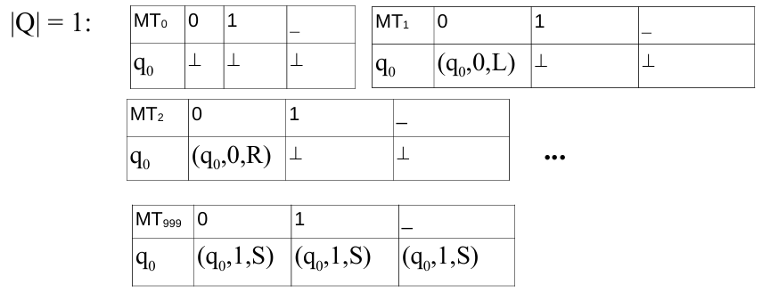
For example, if we start with a single-state TM (where ), operating on a simple alphabet , the total number of possible transition functions is giving us 1000 unique one-state TMs, which we can label as . For TMs with two states, the possibilities increase significantly due to the expanded transition table. Specifically, with two states, the count becomes unique two-state TMs, each indexed sequentially after the one-state TMs.

Through this approach, we establish an effective enumeration , where is computable by an algorithm, meaning a TM can execute it. With this enumeration, we can also produce the TM corresponding to any natural number and, conversely, identify the index of any given TM . The position of in this enumeration is called the Goedel number of , and this enumeration process is known as goedelization.

For simplicity in discussing computability, we generally identify each TM by its Goedel number and, by convention, consider every problem as a function . In this context, denotes the function computed by the ^th TM, corresponding to the ^th entry in our enumeration. This framework enables us to map computational problems to specific TMs and analyze them within a structured, numeric sequence, providing an organized approach to studying computability and the limits of algorithmic problem-solving.

Second fact: Universal Turing Machine (UTM)

A crucial concept in the theory of computation is the existence of a Universal Turing Machine (UTM).

Definition

The UTM is a special kind of Turing machine capable of simulating any other Turing machine. Formally, the UTM computes a two-variable function , where represents the function computed by the ^th Turing machine on input .

At first glance, the UTM appears distinct from the family of TMs because while depends on a single variable , and is a function of two variables, (representing the program) and (the input to the program).

However, this discrepancy is resolved by recognizing that pairs of integers can be effectively enumerated and mapped to a single integer. A common bijection between (the set of integer pairs) and is provided by the pairing function:

This function uniquely encodes a pair as a single number . Its inverse, , decodes back into . Since both and are computable functions, we can translate the problem of simulating into one involving a single variable, . Thus, the UTM can be redefined to compute a function , which is equivalent to under this encoding.

The operation of the UTM can be outlined as follows:

Steps

1. Given an input , the UTM computes to retrieve the pair .
2. Using , the UTM reconstructs the transition function of the ^th Turing machine . This is achieved by applying , the inverse of the enumeration function , which maps natural numbers to TMs.
3. The UTM stores the transition function of on a designated portion of its tape.
4. On another portion of the tape, the UTM encodes the initial configuration of operating on input .
5. The UTM then simulates step-by-step.

• If halts on , the UTM outputs .
• If does not halt, the UTM will not produce an output.

To facilitate these steps, special symbols such as , $$$, and others are encoded as binary strings, ensuring that all components of the simulation are manageable within the binary framework of a Turing machine.

This abstract process highlights an important distinction between a standard TM and a UTM.

• A standard TM is analogous to a computer with a single, fixed program—it always executes the same algorithm and computes the same function.
• In contrast, the UTM is akin to a modern computer with memory-stored programs. The program determines the algorithm to be executed, while serves as the input to that algorithm.

Which Problems can be Solved Algorithmically?

The question of “Which problems can be solved algorithmically?” leads us into a profound exploration of the nature of computable functions and their relationship with definable problems. To answer this, it is essential to understand the size and scope of the sets of all functions, computable functions, and problems that can be defined or solved.

How Many Functions Exist?

Let us begin with the set of all possible functions , where denotes the set of natural numbers. The cardinality of this set is immense. To illustrate this, consider the subset of functions , which can be mapped to subsets of .

This mapping demonstrates that the cardinality of all functions is at least as large as the power set of , , whose cardinality is , the cardinality of the continuum. Thus, the set of all functions from to is uncountably infinite.

How Many Computable Functions Exist?

In stark contrast, the set of computable functions , which are precisely the functions that can be computed by some Turing machine, is countably infinite. This is because Turing machines themselves can be enumerated: there exists a bijection between the set of Turing machines and , which naturally induces an enumeration of computable functions. While this mapping is not one-to-one—many Turing machines can compute the same function—the computable functions form a countable set.

Given that (the cardinality of the natural numbers) and (the cardinality of the continuum), we conclude that:

This inequality implies that the vast majority of functions are not computable. Consequently, “most” problems cannot be solved algorithmically.

This observation raises a natural question: Is the fact that most functions are not computable a significant limitation? To address this, we must consider how problems are defined. Problems are typically described using strings in a language, such as:

• “Find the number that, when multiplied by itself, equals ”

A language over an alphabet corresponds to a subset of , the set of all finite strings over . Since is countable, the set of all definable problems is also countable. Thus, both the set of definable problems and the set of algorithmically solvable problems are countable. This countability suggests the tantalizing possibility that every definable problem might also be solvable, or at least that the two sets could have substantial overlap. However, it is important to emphasize that:

That is, every problem that can be solved algorithmically must first be definable, but not every definable problem is necessarily solvable.

It is worth noting that Turing machines do more than compute functions; they also define functions.

Which Problems can be Solved?

One of the most fundamental questions in computation is understanding the limits of what can be algorithmically solved. Among these limits lies the problem of termination, which has significant practical implications.

The Termination Problem

Consider the scenario where:

1. A program is written.
2. Input data is provided to this program.
3. It is known that, in general, the program may not terminate (it may enter an infinite loop).

The question is: Can we determine, in advance, whether the program will terminate for a given input?

This question, reformulated in terms of Turing machines, can be expressed as follows: Define a function such that:

Here, represents the function computed by the ^th Turing machine on input , and denotes that the TM does not terminate.

The question then becomes: Is computable?

There does not exist a Turing machine that can decide, for all programs and inputs, whether the program will terminate.

This result highlights an intrinsic limitation of computation: a computer cannot reliably predict if a program will run indefinitely on a given input. While computers can easily identify syntactic errors like a missing brace, determining the termination of an arbitrary program is undecidable.

To illustrate this, consider two problems:

• Decidable problem: Determining whether an arithmetic expression is well-parenthesized. This is a solvable problem, and a TM can compute it.
• Undecidable problem: Determining whether a program will run indefinitely on a given input. This is algorithmically unsolvable.

This result does not stand alone—there are many other undecidable problems that we will encounter as we explore the boundaries of computation.

Proof of the Termination Problem’s Undecidability

The proof uses a diagonalization argument, a technique that has its origins in Cantor’s theorem, which demonstrates that .

---

Let us assume, for contradiction, that is computable. This leads to a contradiction as follows:

1. Define :

Suppose is a total, computable function.

2. Define using :

   Here, flips the “yes” answer () into nontermination () and the “no” answer () into termination ().

   By modifying the TM that computes , it is straightforward to construct a TM that computes . Thus, is computable.

3. Diagonalization: If is computable, there exists some such that . In other words, . Consider :

   • If , then , meaning . This is a contradiction because implies terminates.
   • If , then , meaning . This is also a contradiction because implies does not terminate.

   In both cases, we reach a contradiction.

The assumption that is computable is false. Hence, the termination problem is undecidable.

Corollaries and Extensions of the Halting Problem

1. The Uncomputability of h(x)

The halting problem establishes the existence of uncomputable functions, and a natural corollary is the uncomputability of the predicate , which determines whether a function applied to itself halts.

Specifically:

This predicate is not computable. This result follows directly from the proof of the uncomputability of , where:

since is a special case of with . Thus, .

However, the uncomputability of is not strictly a consequence of the uncomputability of . In general, the solvability of a specific case of an unsolvable problem does not imply that the broader problem is solvable. Conversely, a special case of a solvable problem is always solvable, while a generalization of a solvable problem might become unsolvable.

2. Totality Problem (k(y))

Another significant unsolvable problem concerns the function , which determines whether a function is total:

This problem asks whether a program halts for every possible input rather than for a specific input.

From a practical perspective, the totality problem is more significant than the halting problem: while the halting problem considers a single program-input pair, the totality problem requires verifying termination for all possible inputs.

Testing a program on a set of inputs cannot guarantee a solution to the totality problem:

• If one can identify a specific input such that , it conclusively proves that is not total.
• However, even exhaustive testing over a large set of inputs cannot guarantee that is total, as there may always exist some input for which .

This asymmetry also applies in the reverse case: if it can be proven that is total, then there is no doubt that for any .

The unsolvability of is a direct consequence of Rice’s Theorem, which states that

Rice's Theorem

any non-trivial property of the function computed by a Turing machine is undecidable.

Since characterizes the set of total functions, it is a non-trivial property, and thus, it is uncomputable.

While the halting problem addresses whether a program terminates for a specific input , the totality problem involves a universal quantifier:

• Halting Problem (): Is there a guarantee that halts for input ?
• Totality Problem (): Does halt for every possible input?

The universal quantification in the totality problem makes it fundamentally distinct and often more challenging from a computational perspective. Testing alone is ineffective for resolving totality.

The totality problem illustrates a deeper limitation of computation:

• Even when a program behaves correctly over many inputs, it is impossible to guarantee totality without encountering undecidability.
• This insight highlights the importance of formal methods in software verification, especially when designing systems where totality (e.g., guaranteed termination) is critical.

Proof of the Uncomputability of

The function is defined as:

This function identifies whether , the function computed by the ^th Turing Machine (TM), is total (halts for all inputs). The goal is to prove that is uncomputable.

---

1. Hypothesis
   Assume, for the sake of contradiction, that is computable. By definition, is a total function (it provides an output for any ).

2. Defining : A Function Enumerating Total Functions
   Define as follows:

   • gives the Gödel number (or index) of the ^th TM in the enumeration that computes a total function.
   • is constructed algorithmically:
     • Compute until the first such that .
     • Let .
     • For , find the second such that , and so on.
   • Since there are infinitely many total functions, is well-defined for all , making a total function.
   • Furthermore, is strictly monotonic: .

3. Invertibility of
   Since is strictly monotonic, it is invertible on its domain. Let denote the inverse of , defined only for values of that are Gödel numbers of total functions.

4. Defining a New Function
   Define the function as:

   where is the ^th TM’s output on input , indexed by . By construction:

   • is total (as enumerates only total functions).
   • Hence, is also total and computable.

5. Diagonalization

   • By the definition of TMs, there exists some such that . In other words, for all .
   • Since , substituting gives:
   • From the assumption , it also holds that:

6. Contradiction

   • Substituting , we find:
   • But , so:
   • This creates a contradiction because:

Knowing that a Problem is Solvable does not Mean Being Able to Solve it

A fundamental concept in computational theory is that the solvability of a problem does not guarantee our ability to solve it. This distinction arises frequently in mathematics and theoretical computer science, where proofs of existence often demonstrate that a certain solution or mathematical object exists without providing any constructive method to find it. Such proofs are referred to as non-constructive proofs, which are theoretical in nature but lack an explicit algorithmic process to exhibit the solution.

In the context of Turing Machines, a problem is said to be solvable if there exists at least one TM capable of solving it.

However, this theoretical guarantee does not imply practical computability in all cases. For some problems, we may know that a TM capable of solving the problem exists, but we might not know how to construct it. Even if we have a set of TMs that contains the correct one, we may lack the means to identify which TM in the set solves the problem. This gap highlights the difference between theoretical solvability and practical implementation.

Example

To better understand this concept, consider a simple example involving closed, yes-or-no questions, where the answer is independent of any input or parameters. Questions such as “Is the number of atoms in the universe equal to ?” or “Will the perfect chess game always end in a draw?” illustrate this point.

These are examples of problems where the answer is definitively either “yes” or “no,” even though we may not currently know which one. The answer to such questions can be associated with a constant function, where one encodes TRUE = 1 and FALSE = 0. For example:

Both functions are trivially computable because they are constant functions. This means that whatever the answer to the question, it is theoretically computable, even if the actual solution remains unknown.

To generalize this idea, consider the halting problem function, , which is defined as follows:

Here, determines whether the ^th TM halts when given input .

Example

For instance, asks if TM halts on input , while evaluates if TM halts on input . Each of these specific instances represents a solvable problem in the sense that the answer to each question is definitively either or .

However, despite the theoretical solvability, we cannot always determine the solution for arbitrary arguments and . This limitation stems from the fact that there is no general algorithm capable of solving the halting problem for all possible inputs due to its undecidability.

Thus, while the solvability of a problem guarantees the existence of a solution, it does not necessarily imply that the solution is accessible or constructible.

Decidability and Semidecidability

In computational theory, we often analyze problems by framing them as binary decision problems. A binary decision problem is expressed in the following form:

Problem: Given a set and an element , is ?

This formulation allows us to view problems as languages, where each problem corresponds to a set of natural numbers or strings (depending on the context).

Definition

The characteristic function (or predicate) of a set is a total function that determines membership in . It is defined as:

By definition, is total, meaning it produces a value for every input .

The nature of this function is fundamental to determining whether a set is recursive or recursively enumerable.

Definition

A set is called recursive (or decidable) if and only if its characteristic function is computable by a Turing Machine (TM).

This means there exists an algorithm that, given any , always terminates with a correct yes-or-no answer about whether .

For this reason, solvable problems are often referred to as decidable problems.

In practical terms, for decidable problems:

• A TM halts on all inputs and produces the correct decision for any .
• The decision process is guaranteed to conclude in finite time, regardless of whether .

Definition

A set is recursively enumerable (RE) (or semidecidable) if it satisfies one of the following equivalent conditions:

1. is the empty set ().
2. is the image of a total, computable function , known as the generating function of . Formally: which means .

This definition emphasizes the algorithmic nature of semidecidable sets. The term recursively enumerable arises because the elements of can be systematically enumerated by applying to successive inputs.

Semidecidability

The concept of semidecidability can be understood intuitively:

• If , there exists a process to enumerate the elements of , and eventually will be found. This allows the procedure to terminate with a “yes” answer.
• However, if , the enumeration of elements will continue indefinitely without ever reaching . Consequently, no conclusion is reached, and the process does not terminate.

Example

For example, consider the question “Is ?“.

• If belongs to , enumeration ensures that will appear in the list of elements generated by , confirming membership.
• Conversely, if , the procedure offers no means of certainty, as the absence of cannot be conclusively determined.

This limitation highlights the distinction between decidability and semidecidability:

• Decidable problems guarantee a definitive answer (yes or no) for every input in finite time.
• Semidecidable problems guarantee a “yes” answer if , but no such guarantee exists for a “no” answer if .

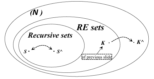
In the theory of computation, decidable and semidecidable sets (or problems) are crucial for understanding the limits of algorithmic computation.

Theorem A:

If is Recursive, then is RE (Recursively Enumerable).

This theorem establishes that every recursive (decidable) set is also recursively enumerable (semidecidable). Intuitively, this makes sense because decidable problems are fully solvable, while semidecidable problems are only partially solvable (i.e., solvable when the answer is “yes”). Therefore, being decidable implies being semidecidable, but not vice versa.

Proof

If , it is RE by definition, since an empty set can be trivially enumerated (no elements to produce).

---

Now consider the case where . Let be the characteristic predicate of , defined as:

Since , there exists some such that . We construct a generating function as follows:

This function is total and computable because is computable. Furthermore, enumerates , meaning that . Therefore, is RE.

This is a non-constructive proof. While we know that is RE if , we do not necessarily know whether is non-empty.

Theorem B

A Set is Recursive if and only if both and are RE

This result is central to understanding decidability. It states that a set is recursive if its complement is also RE. In other words, two semidecidabilities make a decidability: the ability to semidecide both and ensures that is fully decidable.

Proof

This theorem can be split into two implications:

1. If is recursive, then both and are RE.

   • Since is recursive, its characteristic function is computable. This also means , the characteristic function of , is computable because .
   • Hence, is recursive and, by Theorem A, recursively enumerable.

2. If both and are RE, then is recursive.

   • If and are both RE, we can construct a combined enumeration that determines whether any given belongs to or .
   • Specifically, let enumerate and enumerate . For any , construct an interleaved enumeration: . If appears in an odd position, ; if it appears in an even position, . This procedure guarantees that can be computed, making recursive.

Corollary

The class of recursive sets (languages, problems) is closed under complement because if is recursive, so is .

While recursive sets are closed under complementation, recursively enumerable sets are not. If RE sets were closed under complement, all RE sets would be recursive because both and would then be RE for any RE set . However, this is not the case, as shown by examples like the Halting Problem.

Special Results

1. Characterization of RE Sets: A set is RE if and only if , where is a computable, partial function. Alternatively, is RE if and only if , where is a computable, total function.

2. Existence of Non-Recursive RE Sets: Consider the set , where denotes whether Turing Machine halts on input . This set is semidecidable because we can enumerate for which , but it is not decidable because the characteristic function is not computable.

The Mighty Rice Theorem

Rice’s Theorem is a fundamental result in computability theory that has far-reaching consequences in understanding the decidability of problems concerning the behavior of Turing Machines (TMs). It reveals that almost all non-trivial properties of the functions computed by TMs are undecidable.

Rice's Theorem

Let be a set of computable functions. Define the set as:

where is the function computed by the Turing Machine (associated with index ).

Rice’s Theorem states that is decidable if and only if is either the empty set () or the set of all computable functions (). In all other cases, where contains some computable functions but not others, is undecidable.

The theorem asserts that any non-trivial property of the functions computed by TMs is undecidable. A property is trivial if it applies to either none of the computable functions or all of them. For any property of the function’s behavior—such as its output range, correctness, or equivalence—the problem of determining whether a TM satisfies the property is undecidable unless the property is trivial.

Rice’s Theorem directly implies the undecidability of many interesting and practically significant problems, such as:

1. Program Correctness:
   Determining whether a program solves a specific problem (i.e., whether ) is undecidable. Here, , a non-trivial set, making undecidable.

2. Program Equivalence:
   Given two programs and , determining whether (i.e., whether they compute the same function) is undecidable. The associated set makes the problem non-trivial.

3. Specified Function Properties:
   Determining whether a program computes a function with specific characteristics is undecidable, such as:

   • A function whose image contains only even values.
   • A function whose image is finite or bounded.
   • A function with certain structural properties, like periodicity or symmetry.

4. Other Behavioral Properties:
   Whether a program halts on all inputs, produces certain types of outputs, or has specific runtime behavior is undecidable.

Rice’s Theorem provides a systematic way to reason about the decidability of problems without the need for new proofs for each case. Here’s how we can evaluate a problem:

Algorithm

1. Decidability:
   If we can design an algorithm that always terminates and provides the correct answer for all inputs, the problem is decidable.

2. Semidecidability:
   If there exists an algorithm that terminates when the answer is “yes” but may run indefinitely otherwise, the problem is semidecidable.

3. Proving Undecidability:

   • Use Rice’s Theorem: If the problem concerns a property of the function computed by a TM and the property is non-trivial, it is undecidable.
   • Reduce from a known undecidable problem: Many undecidability proofs leverage reductions, showing that solving one problem would solve another undecidable problem, leading to a contradiction.

Rice’s Theorem is immensely powerful because it provides a general framework to classify a wide range of problems as undecidable.

Reduction Problem

Reduction is a fundamental tool in computability theory and theoretical computer science, allowing us to establish the (un)decidability of complex problems. By transforming one problem into another, we can leverage existing knowledge about a problem’s solvability or unsolvability to infer similar properties about the problem at hand.

Problem reduction is the process of algorithmically transforming an instance of one problem into an instance of another problem , such that solving allows us to solve .

Definition

Formally, suppose we want to solve . If we have a total, computable function such that: then we can solve by solving , where . This establishes a reduction from to , denoted as .

Two Directions of Problem Reduction

1. From Decidability to Decidability: If is decidable and can be reduced to , then is also decidable.
2. From Undecidability to Undecidability: If is undecidable and can be reduced to , then is also undecidable. This works because solving would imply a solution for , contradicting the undecidability of .

Example of Problem Reduction: Multiplication

A trivial example of reduction is the computation of a product using operations like addition, subtraction, division by , and squaring. Using the formula:

we reduce multiplication to the set of operations {addition, subtraction, division by 2, squaring}.

Applications of Problem Reduction

1. Halting Problem:
   The undecidability of the Halting Problem is often used as a starting point for proving the undecidability of other problems. For instance:

   • The Halting Problem asks whether a given Turing Machine halts on an input .
   • If one could solve certain program properties, such as “does a program access an uninitialized variable?”, then one could solve the Halting Problem by reduction.

2. Uninitialized Variable Access:
   Consider reducing the Halting Problem to the problem of determining whether a program accesses an uninitialized variable.

   • Transform into :

     P^:
     begin
       var x, y: … 
       P; 
       y := x; 
     end

   • Here, and are new variables not used in .

   • If terminates, the assignment accesses , which is uninitialized. Thus, solving the uninitialized variable access problem for would solve the Halting Problem for , which is impossible.

   This demonstrates that detecting uninitialized variable access is undecidable.

3. Run-Time Errors:
   The same technique applies to proving the undecidability of common program execution properties, such as:

   • Array index out-of-bounds.
   • Division by zero.
   • Dynamic type incompatibility.

   While many problems are undecidable, they can often be semidecidable. For example:

   • Halting Problem: If a Turing Machine halts, we can eventually verify this by observing its termination.
   • Runtime Errors: Consider the problem of detecting a division by zero in a program . If ever executes a division by zero on an input , we will eventually observe it during execution.

   However, if does not halt on , it is unclear whether would execute a division by zero on any other input . Thus, the problem is semidecidable:

   • Positive Case: If a division by zero occurs, it is detected.
   • Negative Case: If no division by zero occurs, the program may run indefinitely without yielding a conclusion.

Theorem: Abstract Formulation of Semidecidability

The theorem provides a general framework for understanding semidecidable sets, particularly in the context of computable functions and runtime errors. It states:

Theorem

The set of values for which there exists a such that is semidecidable.

Here, represents the index of a Turing Machine (TM), and the problem’s input is the TM index .

Sketch of the Proof: Semidecidability via Dovetailing

The proof hinges on the “dovetailing” technique, a systematic method for simulating multiple computations in parallel, ensuring eventual discovery of a solution if one exists. Here’s how it works:

1. Initial Computation: Begin by simulating the computation .
   • If , the computation halts, and the answer is positive.
2. Challenge: What if does not terminate?
   • In this case, it’s possible that , or for some other value , .
3. Dovetailing Strategy: To handle this, adopt the following approach:
   • Simulate one computation step of .
   • If it does not halt, simulate one step of .
   • If does not halt either, simulate two steps of , then one step of , then two steps of , and so on.
   This sequence can be visualized as:

4. Guarantee: If there exists a such that , the dovetailing strategy ensures that the computation will eventually reach enough steps to find it.

Implications of the Theorem

1. Significance for Runtime Errors:
   The theorem highlights that many sets associated with runtime errors in programs are semidecidable. For example:
   • Detecting the presence of an error (e.g., a division by zero) is semidecidable because we can eventually observe the error during computation.
   • However, the absence of errors (i.e., correctness of a program) is not semidecidable.
2. Complement of Semidecidable Sets:
   • If a set is semidecidable (), its complement is not semidecidable if .
   • This follows because if both and were semidecidable, then would be decidable, contradicting .

The theorem has profound implications for software testing and verification:

• Error Detection: Testing can demonstrate the presence of errors in a program (since errors, if they exist, are semidecidable).
• Error Absence: Testing cannot prove the absence of errors. This is because the set of error-free programs is the complement of the set of erroneous programs and is not semidecidable.

This principle was famously articulated by Edsger Dijkstra:

Quote

“Testing can prove the presence of errors, but not their absence.”

Edsger Dijkstra

The theorem also provides a systematic approach to prove that a problem is not RE (recursively enumerable):

• If , then its complement must be RE.
• Conversely, if is not RE, it implies that is not semidecidable either.

This insight allows us to demonstrate the non-semidecidability of a set by showing that its complement is semidecidable.