graph TD
	UR((User<br>Requirement))
    DBs((Internal<br>DBs))
    IS((Further<br>Info Sources))
    SS[Source Selection]
    TA[Translation into a<br>common conceptual model]
    SA[Source Analysis]
    CS[Conceptual Schema<br>integration]
    CD[Conceptual Design]
    LD[Logical Design]
    PD[Physical Design]

    UR --> SS
    DBs --> SS
    IS --> SS

    subgraph Analysis
        direction LR
        SS --> TA
        TA --> SA
    end

    subgraph Integration
        SA --> CS
    end

    subgraph Design
        direction LR
        CS --> CD
        CD --> LD
        LD --> PD
    end
To effectively study data warehousing and its design process, it is crucial to understand the flow from user requirements to physical design. The process begins with gathering user requirements, which serves as the foundation for the entire data warehousing initiative. This initial step is pivotal as it captures the needs and expectations of the users who will ultimately utilize the data warehouse. After this, we move into the analysis phase, which involves several key activities.
In the analysis phase, the first task is source selection, where we identify and evaluate potential data sources, including internal databases and further information sources. This stage is essential because the selected sources will determine the quality and relevance of the data included in the warehouse. Following source selection, the next step is to translate the gathered user requirements into a common conceptual model. This process allows us to create a unified representation of the data that is both understandable and actionable. The source analysis then occurs, where the selected data sources are thoroughly examined to ascertain their compatibility and relevance for integration.
The integration phase is critical as it involves the amalgamation of the conceptual schemata derived from the analysis. This stage is where the various models and structures of the data sources are integrated into a coherent framework that can support the design of the data warehouse.
Next, we move into the design phase, which consists of three main components: conceptual design, logical design, and physical design. The conceptual design translates the integrated schemata into a high-level framework that defines the structure of the data warehouse without delving into implementation details. The logical design then refines this framework into a more detailed schema, taking into account the logical relationships between different data entities. Finally, the physical design translates the logical schema into a concrete structure that outlines how the data will be physically stored in the database management system (DBMS).
It is important to note that data warehouses typically operate on a multidimensional model, which facilitates complex queries and analytical processing.
Unlike traditional databases that utilize the Entity/Relationship model, data warehouses require a different conceptual approach. The absence of a universal conceptual model for data warehouses means that each implementation may vary significantly based on the specific requirements and the context of use.
Throughout this entire process, factors such as workload, data volume, and the chosen DBMS play significant roles in shaping both the logical and physical designs. The reconciled schema encapsulates the decisions made during these stages, ensuring that the final structure meets user requirements while optimizing performance and storage efficiency.
graph TD
  A[[Conceptual Design]]
  B[[Logical Design]]
  C[[Physical Design]]
  D[/Reconciled schema/]
  E[/User requirements/]
  F[/Work load<br>Data volume<br>Logical Model/]
  G[/Work load<br>Data volume<br>DBMS/]
  H((Fact schema))
  I((Logical schema))
  J((Physical schema))

  A --> H --> B --> I --> C --> J
  D --> A
  E --> A
  F --> B
  G --> C
Conceptual Model for Data Warehousing
The conceptual model in data warehousing defines how data is structured to facilitate efficient querying and analysis, particularly through the organization of facts and dimensions. In this model, facts represent quantitative data derived from real-world events, and they interact with dimensions, which are descriptive attributes that provide context to the facts. This setup is foundational to the multidimensional design of a data warehouse.
Facts and Dimensions
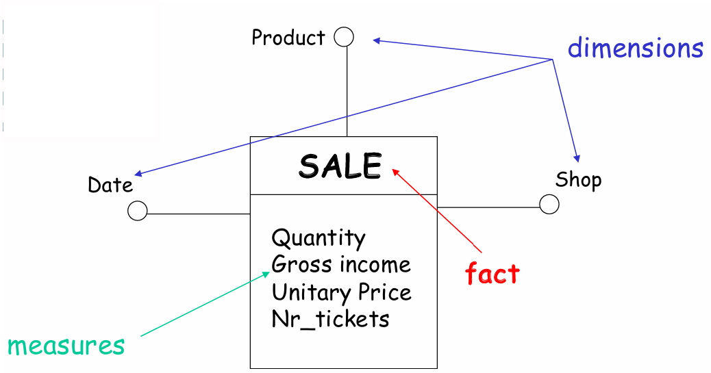
A fact is an
Dimensional Attributes and Hierarchies
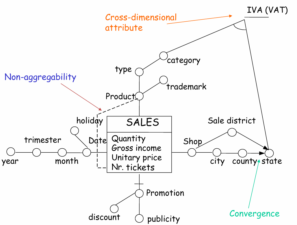
Dimensional attributes are discrete values that represent specific aspects of dimensions, such as product name o sale date. These attributes organize data and enable effective categorization and analysis. A critical feature of dimensional attributes is their ability to form hierarchies. Hierarchies are directed structures resembling trees in which each node is a dimensional attribute, and edges reflect
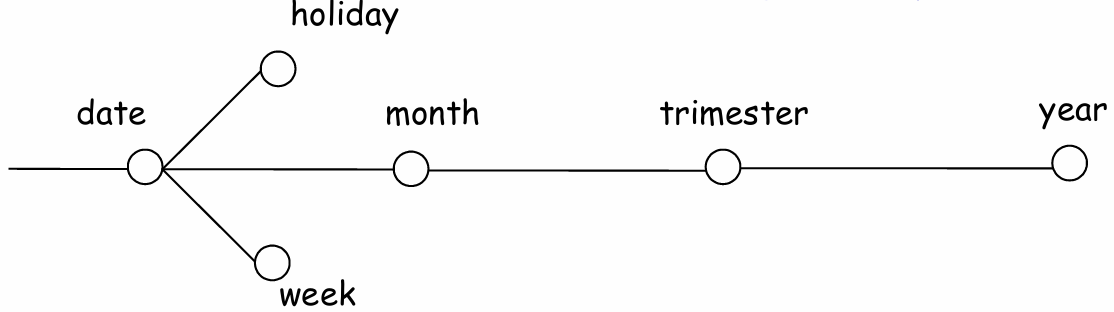
These hierarchies facilitate data aggregation at various levels, enabling users to drill down into details or roll up to broader summaries. For example, in a sales data warehouse, a hierarchy might allow aggregation from individual sales up to monthly totals, quarterly results, or even yearly summaries, enhancing data flexibility for analysis.
Events and Aggregations
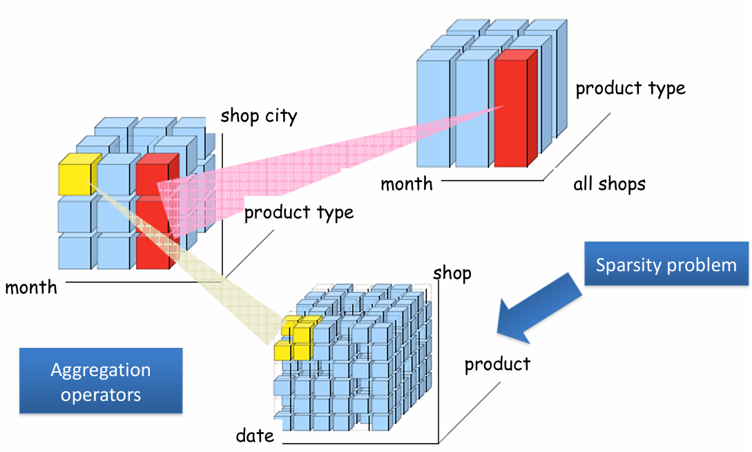
Primary events, represented as fact tuples, capture raw occurrences with the highest level of detail. For instance, a primary event might document a specific sale: “On 10/10/2001, ten ‘Brillo’ detergent packets were sold at BigShop for 25 euros.” This tuple captures precise data points, including the date, product, location, quantity, and sales amount.
Secondary events, by contrast, represent aggregated data derived from primary events. These aggregates allow analysts to view data at coarser granularity, enabling them to observe patterns and trends. For example, the sales for “Brillo” detergent packets might be aggregated by month or city, transforming a collection of daily transactions into monthly sales totals for each product and location. A secondary event could be described by the tuple (city: ‘Rome’, product: ‘Brillo’, month: 10/2001), indicating all sales of ‘Brillo’ in Rome during October 2001.
Descriptive Attributes
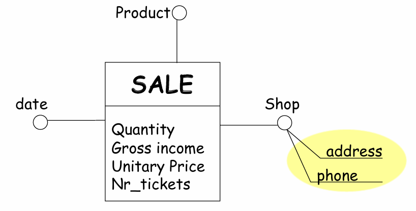
Descriptive attributes provide additional context for dimensional attributes. They are determined by the dimensional attribute with which they are associated, adding depth to the analysis. For instance, a shop attribute could be described by its address and phone number attributes, enriching the data with more detailed information.
Descriptive attributes are essential for enhancing the granularity and specificity of data analysis, enabling users to explore relationships and patterns more comprehensively.
Optional Edges and Dimensions
Fact schemas can include optional edges, which offer flexibility by allowing certain associations to be excluded when unnecessary. Similarly, optional dimensions accommodate specific scenarios in which data only applies under particular conditions.
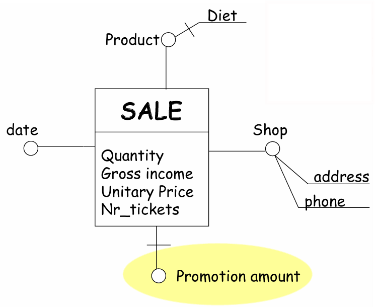
For example, the dimension ‘Promotion amount’ would only be relevant for products currently on promotion, so the data warehouse schema can selectively include this dimension where applicable, optimizing storage and processing for these cases.
Cross-Dimensional Attributes
Cross-dimensional attributes are derived values based on multiple dimensions. These attributes enable complex calculations that span more than one dimension. For example, the IVA (VAT) might depend on both the product category and the country. Such attributes enrich the data model by providing insights across dimensions without requiring complex joins or additional data retrieval steps.
Convergence in Hierarchies
Convergence in data warehousing hierarchies refers to situations where two or more paths connect the same dimensional attributes within a hierarchy structure. This allows for flexible ways to navigate the data depending on different organizational or analytical needs. In a typical hierarchical path, convergence can occur when there are alternative routes between two levels.
Example
For example, consider a retail data model where we have two paths leading to the attribute ‘state’: one through a direct geographic hierarchy, such as
, and another through a sales-oriented path, such as . Here, both routes converge on state, enabling analyses based on either geography or sales management structures.
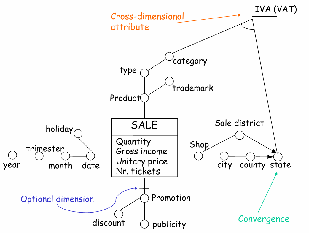
This convergence supports versatile querying and reporting, as users can analyze data by geographical hierarchy or by business organization, depending on the analytical requirement. Each path may represent different functional dependencies within the model, allowing greater flexibility and adaptability within a unified schema.
Hierarchy Sharing
Hierarchy sharing is a modeling shorthand used to represent instances where portions of a hierarchy overlap within a fact schema. This method avoids redundancy by enabling shared branches to act as common components across different hierarchies. For example, if several facts share a dimension like phone number, hierarchy sharing allows this dimension to be represented only once, despite being referenced by multiple facts. When hierarchy sharing starts from a dimension attribute, it is necessary to label incoming edges with roles to maintain clarity on functional dependencies and ensure data integrity.
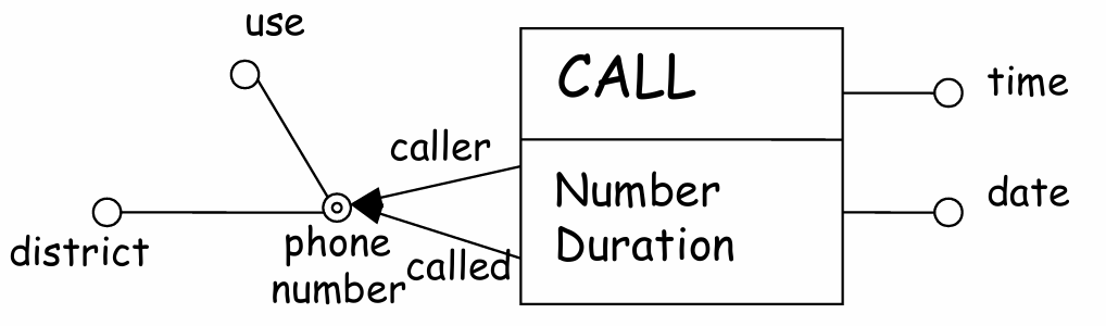
The functional dependency requirement mandates that each branch maintain a consistent functional relationship with the root, preventing ambiguity in shared structures. Hierarchy sharing reduces complexity and storage requirements in large-scale data warehouses by avoiding duplicative hierarchies while ensuring all paths to dimensional attributes are clear and efficient.
Multiple Edges in Fact Schemas
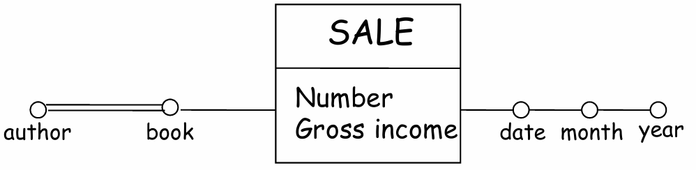
In a well-designed fact schema, a functional dependency must exist between each fact and its associated dimensions, ensuring each fact uniquely corresponds to a combination of dimensional values. However, some dimensions may relate through a many-to-many relationship, represented by multiple edges in the schema. For instance, a product may belong to multiple categories or apply to multiple promotions. These multiple edges represent complex relationships that deviate from the standard one-to-many structure and require special handling during the logical design phase to ensure they align with the data warehouse’s analytical structure.
Aggregability in Data Warehousing
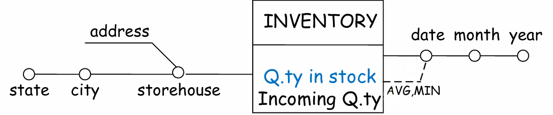
In data warehousing, aggregability refers to the ability to combine values associated with primary events (individual records) into values for secondary events (aggregated records) using specific aggregation operators. Aggregability ensures that measures (quantitative values) can be meaningfully summarized across certain dimensions, like time or location, to create insights at different levels of granularity.
When discussing measures, it is essential to understand that not all are fully aggregable across all dimensions. A measure is considered additive along a dimension if it can be freely aggregated using the SUM operator without risking inaccurate or misleading results. For instance, the “amount sold” measure is additive concerning time and space, meaning that sales quantities can be summed across days or regions for a meaningful aggregate. In contrast, certain measures, such as “quantity in stock” (a level measure), are non-additive with respect to time, as summing stock levels across multiple periods does not yield meaningful results. Instead, such measures are typically aggregated using AVG (average) or MIN (minimum) to represent them accurately across time.
Examples of Aggregability and Non-Aggregability
A practical example of aggregability is seen with “quantity in stock.” If one wishes to observe stock levels over a month, using the
SUMoperator would be inappropriate because it could inaccurately inflate stock values, as each day’s stock level reflects the same inventory held at different times. Instead, using theAVGoperator would provide a more realistic monthly stock level, while theMINoperator might indicate the lowest stock observed during that month.On the other hand, consider the “number of tickets” measure, representing the count of transactions. This measure is non-additive and generally non-aggregable with respect to the product dimension. In a retail setting, a ticket (receipt) can include multiple products and even multiple instances of the same product type, creating a many-to-many relationship between products and tickets. For instance, if one aggregates the ticket count by product type, tickets that include multiple units of the same product type might be counted multiple times.
To illustrate this, suppose we have the following ticket data:
Ticket Product Type S1 P1 T1 S1 P2 T1 S2 P1 T1 S2 P3 T2 Here, if we calculate the number of tickets containing products of type T1 by simply summing them, we end up with a result of 3, as each appearance is counted. However, the true count of unique tickets is 2 because tickets S1 and S2 each contain multiple products of type T1. Such double-counting errors make the
SUMoperator inappropriate for this type of aggregation, highlighting the need for careful consideration of aggregation operators.
Empty Fact Schemata
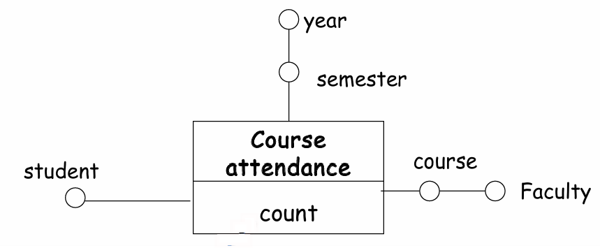
A fact schema is considered empty if it contains no measures to analyze. In such cases, a default measure—usually a simple count—is implied. This count measure indicates the number of occurrences within the schema, providing basic insight into the volume or frequency of events even when specific measures are absent. An empty fact schema is useful in scenarios where the primary goal is to count occurrences rather than analyze detailed quantitative data.