Designing Data Integration in a Multi database with a Unified Data Model
Data integration within a multi database context involves several critical steps to ensure that disparate data sources can be effectively combined and queried. Below is a comprehensive breakdown of the process, enhanced with additional information to aid in your studies.
Source Schema Identification:
Identify the various schemas of data sources involved in the integration process. Understanding the structure and organization of these schemas is crucial for determining how data can be combined.
Sources may include databases, files, or external APIs, each with its unique schema.
Source Schema Reverse Engineering:
This involves analyzing the data source conceptual schemas to create a detailed representation of the data structures and their relationships.
Techniques like entity-relationship modeling or UML (Unified Modeling Language) diagrams can be used to visualize the schema components.
Conceptual Schemas Integration and Restructuring:
Merge the identified schemas into a unified conceptual schema. This step addresses potential conflicts between the schemas, such as naming inconsistencies or differing data types.
Conflict resolution strategies may include renaming attributes, converting data types, or creating a hierarchy of attributes.
Conceptual to Logical Translation:
Translate the integrated conceptual schema into a logical schema that can be implemented in a specific database management system.
This process often involves normalization, which organizes data to reduce redundancy and improve data integrity.
Mapping Between the Global Logical Schema and Individual Source Schemas:
Define the relationships between the global logical schema and each source schema. This step, also known as logical view definition, is essential for querying the integrated system.
Various mapping techniques, such as Global As View (GAV) and Local As View (LAV), can be employed to facilitate this process:
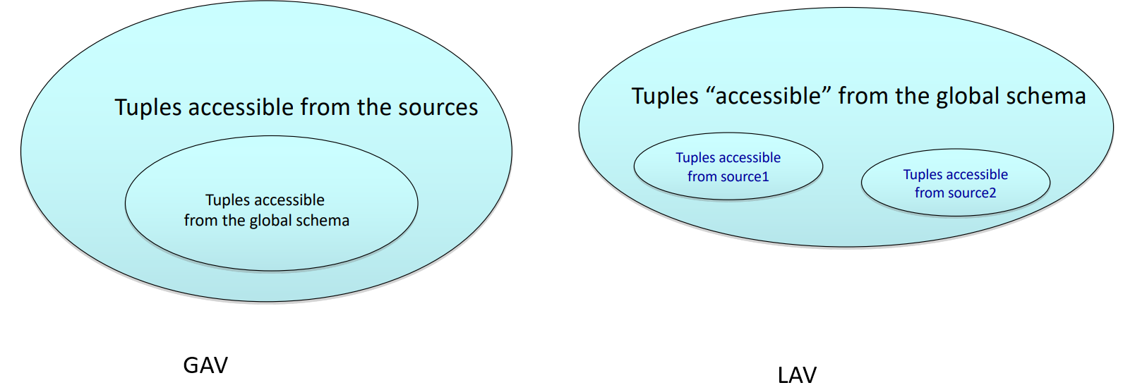
GAV (Global As View): In this approach, the global schema is constructed based on the views of the individual data sources. Each source schema is defined as a view over the global schema.
LAV (Local As View): The global schema is created independently of the source schemas. Instead, each source schema is treated as a view of the global schema, defining how local data fits into the overarching model.
Post-Integration Query Answering through Data Views:
Once integration is complete, queries can be made against the global schema. The system will determine how to retrieve the corresponding data from the individual sources based on the defined mappings.
This may involve translating queries from the global schema context back into the source schemas.
Definition
A data integration system can be formally defined as a triple , where:
: Represents the global schema, which provides a unified view of the integrated data.
: Denotes the set of source schemas from which data is being integrated.
: Consists of the set of mappings that specify how the data from the sources relates to the global schema.
When a query is issued against the integrated system, it is constructed in terms of the global schema . The challenge lies in accurately identifying which pieces of real data in the underlying data sources correspond to the virtual data defined in .
When integrating data from sources that employ different data models (e.g., relational, XML, NoSQL), model transformation may be required. This involves converting data from one model to another to facilitate integration and querying. The mapping techniques discussed earlier (GAV and LAV) remain applicable, but additional considerations may arise depending on the complexity and characteristics of the different data models involved.
Global As View (GAV) Approach
In the Global As View (GAV) approach, the global schema is constructed based on the integration of the individual data source schemas. Each element of the global schema is explicitly defined in terms of queries over the data source schemas, meaning that the global schema is essentially a set of views derived from these sources.
Definition
A GAV mapping consists of a set of assertions that describe how each element of the global schema is computed from the source schemas. Formally, for every element in , there is a corresponding query over the source schemas :
This mapping ensures that each global schema element can be directly traced to specific data in the source schemas, making it easier to understand how global data is derived.
Example
Consider the following table definitions for two data sources, and :
CREATE VIEW GLOB-PROD ASSELECT Code AS PCode, VersionCode as VCode, Version.Name AS Name, Size, Color, Version.Description as Description, CatID, Price, StockFROM SOURCE1.Product, SOURCE1.VersionWHERE Code = ProductCodeUNIONSELECT Code AS PCode, null as VCode, Name, Size, Color, Description,Type as CatID, Price, Q.ty AS StockFROM SOURCE2.Product
we can see how the global schema is constructed by combining data from the two sources. Queries against the global schema will be translated into queries against the source schemas, allowing the system to retrieve the relevant data from the sources. If we have a query like:
SELECT PCode, VCode, Price, Stock FROM GLOB-PROD WHERE Size = "V" AND Color = "Red"
the system will translate this query into the following form to retrieve the necessary data from the source schemas:
SELECT Code, VersionCode, Price, Stock FROM SOURCE1.Product, SOURCE1.Version WHERE Code = ProductCode AND Size = "V" AND Color = "Red"UNIONSELECT Code, null, Price, Q.ty FROM SOURCE2.Product WHERE Size = "V" AND Color = "Red"
The GAV approach works well when the data sources are stable and well-defined, allowing for explicit mappings between the global schema and the source schemas. However, it can be challenging to extend the system when new data sources are added or existing sources change, as the global schema may need to be redefined to accommodate these modifications.
Pros
Cons
Works well with stable data sources
Difficult to extend when new data sources need to be added
Mapping is explicit and clear
Requires redefinition of global schema with source changes
Easier to optimize queries due to fixed mappings
Less flexible for dynamic or evolving data environments
Local As View (LAV) Approach
In the Local As View (LAV) approach, the global schema is designed independently of the data source schemas. Instead of deriving the global schema from the sources (as in GAV), each data source schema is defined as a view over the global schema. The LAV approach allows for more flexibility, especially when new sources are added or existing sources change.
Definition
A LAV mapping is composed of assertions that define how each element in a source relates to the global schema . For every element in the source schema , there is a query that describes how this source element can be viewed in terms of the global schema :
This type of mapping indicates that the content of each source is described as a view over the global schema.
Example
Consider the same example with two data sources, and , and the global schema . In the LAV approach, the source schemas are defined as views over the global schema:
-- SOURCE 1CREATE VIEW SOURCE1.Product ASSELECT PCode AS Code, Name, Description, Warnings, Notes, CatIDFROM GLOB-PRODCREATE VIEW SOURCE1.Version ASSELECT PCode AS ProductCode, VCode as VersionCode, Size, Color, Name, Description , Stock, PriceFROM GLOB-PROD-- SOURCE 2CREATE VIEW SOURCE2.Product ASSELECT PCode AS Code, Name, Size, Color, Description, CatID as Type, Price, Stock AS Q.tyFROM GLOB-PROD
In this case, the source schemas are defined as views over the global schema, indicating how the local data fits into the overarching model. Queries against the global schema will be processed by extracting the relevant data from the sources based on these views.
Query Processing in LAV
One of the key challenges in the LAV approach is query processing. Since queries are expressed in terms of the global schema, but the data resides in the sources, the system must perform reasoning to “invert” the views. Unlike in GAV, where queries can be unfolded directly through simple mappings, LAV requires more complex strategies.
Inverse View Problem:
The system must figure out how to retrieve relevant data from the sources, given that the mapping defines the opposite transformation. This means the system needs to “rewrite” queries in terms of the source schemas and combine the results accordingly.
Query Rewriting and Execution:
Query processing involves constructing a plan that rewrites the query into a set of subqueries to be executed against the sources. The system then combines these partial results to answer the original query. For example, if a query requires data from both SOURCE1.VERSION and SOURCE2.PRODUCT, the system needs to retrieve and integrate this information from both sources.
Reasoning for Query Execution:
Since there is no simple rule for unfolding the views (as in GAV), query execution requires more reasoning. The system needs to infer which data from the sources can satisfy the query based on the global schema, and how to combine results from different sources.
Pros
Cons
Stability and Scalability: Highly modular, suitable for frequently added or updated sources
Complex Query Processing: Inverse transformation needed to retrieve data from sources
Flexibility in Evolving Systems: Simplifies adding new data sources or modifying existing ones
Increased Complexity in Reasoning: Requires significant computational effort and time for query execution
The LAV approach provides greater flexibility and scalability than GAV, particularly in systems where data sources are dynamic and subject to change. However, it comes at the cost of more complex query processing, which requires reasoning and more sophisticated query rewriting techniques. This makes LAV a better choice for environments with evolving data sources, while GAV may be more appropriate for systems with stable and well-defined data sources.
Comparison Between GAV and LAV
GAV
LAV
Mapping quality depends on how well the sources have been compiled into the global schema
Mapping quality depends on how well the sources have been characterized in relation to the global schema
When a source changes or a new one is added, the global schema may need to be redefined
High modularity and extensibility: source changes or additions only require updating the source definition
Query processing is straightforward due to direct mapping
Query processing is more complex and requires reasoning
Example: Query Processing in LAV with Two Data Sources
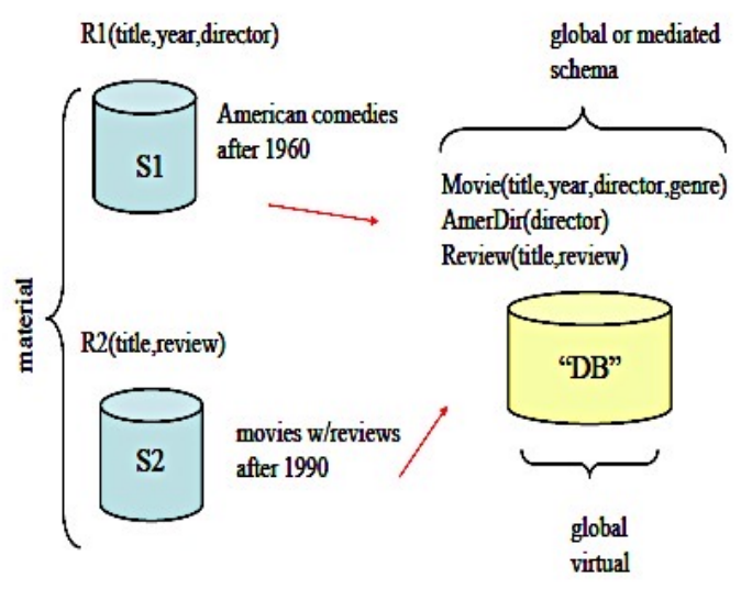
Consider a schema with two sources, S1 and S2, and a global schema G.
S1 contains information about American comedies made after 1960, defined by the view R1(Title, Year, Director).
S2 contains information about movies made after 1990 and their reviews, defined by the view R2(Title, Review).
The global schema G combines data from both sources and is structured as follows:
However, since we are using the LAV approach, the global schema must be “rewritten” in terms of the views from the data sources (S1 and S2). Here’s how the query processing works:
Extract Titles from S1: S1 contains comedies filmed after 1960 with American directors. Therefore, we retrieve all the titles of comedies from R1.
Title ← R1(Title, Year, Director)
Extract Reviews from S2: S2 provides reviews for movies filmed after 1990. We retrieve all the reviews from R2.
Review ← R2(Title, Review)
Join the Results at the Global Level:
At the global level, we now need to join the results from S1 (comedies) and S2 (reviews) based on the movie title.
Due to the limited information in S1 and S2, the result will include only comedies directed by American directors and filmed after 1990, with their corresponding reviews. The information from S2 is incomplete because it only covers movies made after 1990, while the query asks for comedies since 1950. However, since S2 does not contain any data about movies before 1990, it cannot provide reviews for those earlier films.
In general, when using LAV, sources are often incomplete with respect to the global schema. The global schema might represent a broader scope (e.g., all comedies since 1950), but the available data sources may only cover a subset (e.g., comedies after 1960, or reviews after 1990). Therefore, the query results can be incomplete if the data sources do not fully represent the global schema. This is a typical scenario in data integration, where sources provide only partial information about what is expected in the global schema.
Sound, Complete, and Exact Mappings
Definitions
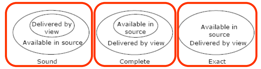
A mapping defined over some data sources is sound when it provides a subset of the data that is available in the data source that corresponds to the definition.
A mapping is complete if it provides a superset of the available data in the data source that corresponds to the definition.
A mapping is exact if it provides all and only data corresponding to the definition: it is both sound and complete.
In GAV (with integrity constraints) the mapping can be exact or only sound. In LAV, the global schema can be defined independently of the sources’ schemata. The mapping can be exact or only complete: what about S2 before, which contained products but not versions, i.e. only a part of the information of the same kind in the global system.
The word “complete” may arise confusion. In the LAV case, the mapping can be exact or only complete, due to the incompleteness of one or more sources. The mapping is complete because the global schema covers the source contents, but the sources are incomplete because they do not cover the data as “expected” from the global schema, which has been defined independently of the source contents.
Operators
Take into account the following tables:
R1
R2
SSN
NAME
AGE
SALARY
SSN
NAME
SALARY
PHONE
123456789
JOHN
34
30K
234567891
KETTY
20K
1234567
234567891
KETTY
27
25K
345678912
WANG
22K
2345678
345678912
WANG
39
32K
456789123
MARY
34K
3456789
where R1 and R2 are two sources. In theses tables, we can perform the following operations:
OuterunionR1 OU R2: the union of the two tables, with the attributes of both tables. If some attributes are missing in one of the tables, they are filled with NULL values.
SSN
NAME
AGE
SALARY
PHONE
123456789
JOHN
34
30K
NULL
234567891
KETTY
27
25K
NULL
345678912
WANG
39
32K
NULL
234567891
KETTY
NULL
20K
1234567
345678912
WANG
NULL
22K
2345678
456789123
MARY
NULL
34K
3456789
JoinR1 JOIN R2: the join of the two tables, with the attributes of both tables. This operator removes all the tuples where the SSN is not present in both tables. If two attributes have the same name, both are present (with different names) in the result.
SSN
NAME
AGE
SALARY1
SALARY2
PHONE
234567891
KETTY
27
25K
20K
1234567
345678912
WANG
39
32K
22K
2345678
OuterjoinR1 OJ R2: the outer join of the two tables, with the attributes of both tables. This operator keeps all the tuples of the first table, and fills with NULL values the attributes of the second table where the SSN is not present in the second table.
SSN
NAME
AGE
SALARY
PHONE
123456789
JOHN
34
30K
NULL
234567891
KETTY
27
NULL
1234567
345678912
WANG
39
NULL
2345678
456789123
MARY
NULL
34K
3456789
GeneralizationR1 Ge R2: the generalization of the two tables, with the attributes of both tables. This operator keeps all the tuples of the first table, and fills with NULL values the attributes of the second table where the SSN is not present in the second table.
SSN
NAME
SALARY
123456789
JOHN
30K
234567891
KETTY
NULL
345678912
WANG
NULL
456789123
MARY
34K
Data Inconsistencies in Data Integration
When integrating data from multiple sources, inconsistencies can arise, leading to challenges in accurately representing real-world entities. These inconsistencies may occur whether a schema exists or not. When different databases contain instances of the same real-world object, discrepancies in the values can occur.
Record Linkage (Entity Resolution): The process of identifying and linking records that refer to the same real-world entities across different datasets. This step is crucial for ensuring that integrated data accurately reflects the entities they represent.
Data Fusion: Once it has been established that two items refer to the same entity, data fusion involves reconciling any inconsistent information between these records. This might include determining which values to retain, merge, or discard based on various criteria or rules.
Data integration frequently requires recognizing strings that refer to the same real-world entities, such as variations in names or addresses.
Example
For example, “Politecnico di Milano” and “Politecnico Milano” might refer to the same institution, while “Via Ponzio 34” and “Via Ponzio 34/5” may represent the same address.
Record Linkage (Entity Resolution)
Regardless of the data model used, identifying when two datasets contain overlapping or identical information is essential. Although the relational data model is often used in these discussions due to its prevalence, the principles are applicable across different models. When fields are distinct, it becomes easier to spot similarities. For example, if one dataset contains “Lonardo” and another contains “Leonardo,” recognizing that “Leonardo” is a campus of Politecnico would allow the system to infer that these represent the same entity.
To effectively perform record linkage, we need to determine which pairs of strings (representing entities) match. Each pair identified as referring to the same entity is called a match.
Similarity Measure:
A similarity measure quantifies how closely two strings (or sets of strings) match, resulting in a value that ranges from 0 to 1. Here:
indicates a perfect match (the strings are identical).
Values closer to 0 indicate a lower degree of similarity.
We can establish a threshold (where ) to determine if two strings match: if , we consider and to be a match.
There are various types of similarity measures used for record linkage:
Sequence-Based Similarity: These measures focus on the sequences of characters in the strings. Examples include:
Edit Distance: Measures the minimum number of edits required to transform one string into another.
Needleman-Wunsch: Used for global sequence alignment.
Smith-Waterman: Used for local sequence alignment.
Jaro and Jaro-Winkler: Focus on the number and order of matching characters.
Set-Based Similarity: These measures treat strings as sets of elements. Examples include:
Overlap: Measures the size of the intersection divided by the size of the union of two sets.
Jaccard: Measures the size of the intersection divided by the size of the union, useful for comparing sets.
TF/IDF: Measures the importance of a term in a document relative to a collection of documents.
Hybrid Similarity: Combines elements of both sequence-based and set-based measures. Examples include:
Generalized Jaccard: An extension of the Jaccard index.
Soft TF/IDF: A modified version of TF/IDF that takes into account similarities in word usage.
Monge-Elkan: A measure designed for comparing two sets of words.
Phonetic Similarity: These measures determine how similar two strings sound when pronounced. An example is:
Soundex: An algorithm for encoding names based on their phonetic similarity.
Edit (Levenshtein) Distance
The edit distance (or Levenshtein distance) is a widely used metric that quantifies the minimum number of operations required to transform one string into another string . The allowable operations are:
Character Insertion: Adding a new character into the string.
Character Deletion: Removing an existing character from the string.
Character Replacement: Changing one character in the string to another character.
The similarity between two strings can be calculated using the edit distance:
Example
For the strings and , the edit distance . This can be achieved through the following operations:
This indicates a high degree of similarity between the two strings.
Calculating for all pairs of strings in a dataset results in a quadratic time complexity, , where is the number of strings. Various algorithms and techniques, such as blocking or canopy clustering, have been proposed to optimize the matching process by reducing the number of comparisons needed.
Set-Based Similarity Measures
Set-based similarity measures treat strings as multisets of tokens. This involves tokenizing the strings and computing a similarity measure based on the resulting sets of tokens. For instance, if we tokenize strings into bigrams (substrings of length 2), the Jaccard similarity can be defined as follows:
Example
For the strings “pino” and “pin” the sets of tokes are:
Using the Jaccard measure:
This indicates a moderate similarity based on the overlap of tokens.
Phonetic Similarity Measures
Phonetic similarity measures assess how alike two strings sound, rather than their literal character composition. One of the most common phonetic algorithms is Soundex. This method generates a four-character code based on the pronunciation of a word, grouping similar-sounding letters under the same code.
Soundex is particularly useful in genealogical research, where names may evolve phonetically over generations.
Example
For example, “Legoff” and “Legough” may yield the same Soundex code, indicating that they sound similar despite being spelled differently.
While Soundex can effectively identify similar-sounding names, it may lead to false positives with common words that sound alike, such as “coughing” and “coffin.” Additionally, phonetic measures are heavily language-dependent, as pronunciation can vary significantly between languages. For instance, the combination “gn” is pronounced differently in English (as in “gnome”) compared to Italian (where it’s pronounced as “ny”).
Record Matching
Record matching is a critical component in data integration and involves identifying and linking records that refer to the same real-world entity across different databases. Various approaches to record matching can be classified into three primary categories:
Rule-based Matching
Learning-based Matching (supervised or unsupervised)
Probabilistic Matching
Before implementing matching techniques, blocking is often employed. This process involves dividing the dataset into smaller subsets (blocks) of item pairs that are likely to match, significantly reducing the number of comparisons needed.
Rule-Based Matching
Rule-based matching relies on manually defined rules that specify conditions under which two tuples are considered a match. For example, two records may be identified as referring to the same individual if they have the same SSN. While straightforward, this method is time-consuming and labor-intensive since rules must be crafted for each attribute.
Example
Given two tables:
SSN
NAME
AGE
SALARY
POSITION
123456789
JOHN
34
30K
ENGINEER
234567891
KETTY
27
25K
ENGINEER
345678912
WANG
39
32K
MANAGER
------------
----------
---
----
--------------
SSN
NAME
AGE
SALARY
PHONE
------------
----------
---
----
--------------
234567891
KETTY
25
20K
1234567
345678912
WANG
38
22K
2345678
456789123
MARY
42
34K
3456789
A potential rule for matching could be:
Here, different similarity measures could be applied to each attribute based on its relevance.
Learning Matching Rules
Learning-based matching can be conducted through supervised or unsupervised methods.
In supervised learning, a classification approach is used where a model is trained on labeled data. The process includes:
Training Phase:
Pairs of tuples are labeled as “yes” (if they match) or “no” (if they don’t).
The system learns the significance of each attribute during this phase.
Weight Definition: Each attribute’s importance in the final matching score is determined.
Application: The learned model is then applied to new pairs of tuples for matching.
While effective, supervised learning requires a substantial amount of training data, which can be a limitation.
In contrast, unsupervised learning approaches, such as clustering techniques, group similar records without the need for labeled training data. This method can identify patterns in the data to suggest potential matches based on inherent similarities.
Probabilistic Matching
Probabilistic matching utilizes probability distributions to model the matching domain, allowing for more nuanced decision-making based on the likelihood of a match.
Pros
Cons
Provides a principled framework that can naturally incorporate diverse domain knowledge
Computationally expensive
Leverages established probabilistic representation and reasoning techniques from AI and database communities
Often challenging to understand and debug matching decisions
Offers a reference framework for comparing and explaining various matching approaches
This approach is beneficial when dealing with uncertain data and can improve matching accuracy by considering the probabilities associated with various matching scenarios.
Data Fusion
Data fusion is the process of integrating and reconciling information from multiple sources to produce a coherent and accurate representation of the same real-world entity. Even after establishing that some data represent the same entity, discrepancies in the information can arise. The challenge then becomes determining how to resolve these inconsistencies.
Resolution Function
Inconsistencies in data can result from various factors, including:
Incorrect Data: One or both of the data sources may contain inaccuracies.
Partial Views: Each source might provide a correct but incomplete view of the entity. For instance:
The total salary might be the sum of the amounts reported by different sources.
A list of authors for a book may not include all contributors.
One source may only provide the first letter of a middle name while another includes the full name.
When reconciling discrepancies, several strategies can be employed. The correct value may be derived from a function of the original values, allowing for a more comprehensive integration. Here are a few examples of how values might be combined:
Summation: Combine values directly, such as total salaries:
Weighted Average: Assign different weights to each value to reflect their reliability:
where .
Maximum or Minimum: Choose the maximum or minimum value from the conflicting data:
Example
Given the following tables representing employee data from two different sources:
Source 1:
SSN
NAME
AGE
SALARY
POSITION
123456789
JOHN
34
30K
ENGINEER
234567891
KETTY
27
25K
ENGINEER
345678912
WANG
39
32K
MANAGER
Source 2:
SSN
NAME
AGE
SALARY
PHONE
123456789
JOHN
34
30K
NULL
234567891
KETTY
27
45K
1234567
345678912
WANG
39
54K
2345678
456789123
MARY
42
34K
3456789
In this scenario, we can fuse the information based on SSN. If we aim to resolve the salary for KETTY, we can sum the salaries from both sources:
Thus, a new integrated table might look like:
SSN
NAME
AGE
SALARY
POSITION
PHONE
123456789
JOHN
34
30K
ENGINEER
NULL
234567891
KETTY
27
70K
ENGINEER
1234567
345678912
WANG
39
54K
MANAGER
2345678
456789123
MARY
42
34K
NULL
3456789
Data fusion is particularly complex in modern contexts where:
There are numerous and heterogeneous data sources, including structured databases, semi-structured sources (like XML), and unstructured data (like text documents).
Different terminologies and operational contexts can create confusion and ambiguity.
Data is often time-variant, especially in environments like the web where information changes rapidly.
Sources may be mobile or transient, adding another layer of complexity to the fusion process.
Data Integration in the Multi database
In a multi database environment, integrating data from various sources is a complex but essential process. This integration allows users to query and manipulate data as if it were coming from a single source, even when it is actually distributed across multiple databases with different schemas and structures.
Wrappers in Data Integration
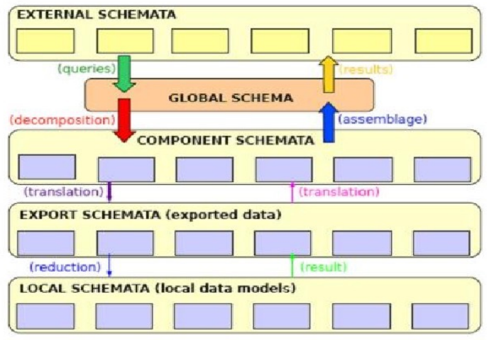
Definition
A Wrapper is a software module that translates queries and results between the global schema and the data source schemata.
Here’s how wrappers function in data integration:
Query Translation: Wrappers convert high-level queries issued to the global schema into specific queries that can be understood by the target data sources. This may involve transforming the syntax or semantics of the query based on the specific database model (e.g., relational, object-oriented, NoSQL).
Result Formatting: Once a query is executed in the data source, the results may be returned in a format that is not directly usable by the application or user. Wrappers translate these results back into a format compatible with the global schema.
Type Conversions: Wrappers can also facilitate type conversions, allowing data types from different databases to be harmonized for consistency and compatibility.
Handling Unstructured Data: While wrappers are relatively straightforward to implement for structured data (like relational or object-oriented data), they become more complex when dealing with unstructured data (like documents, images, etc.). Special techniques may be required to parse and extract meaningful information from such data.
Design Steps for Data Integration in a Multidatabase
To effectively integrate data from multiple sources, the following design steps are typically followed:
Reverse Engineering:
This step involves analyzing the existing databases to produce a conceptual schema that represents the underlying data and its relationships. It helps in understanding how the different sources function and what data they hold.
Conceptual Schemata Integration:
Once the conceptual schemas are produced, the next step is to integrate these schemas. This involves identifying commonalities and discrepancies among the schemas and resolving them to form a unified conceptual model.
Choice of Target Logical Data Model:
After integration, the target logical data model needs to be chosen. This model serves as the basis for the global schema. The global conceptual schema is then translated into this logical model, ensuring that it meets the needs of the application and users.
Definition of the Language Translation (Wrapping):
At this stage, the specifics of how queries and results will be translated between the global schema and individual data sources are defined. This includes specifying the syntax and semantic mappings that wrappers will use.
Definition of Data Views:
Finally, data views are defined to present the integrated data to users or applications. These views encapsulate the complexity of the underlying data sources and provide a simplified interface for data access.