In this study, we do not delve into the detailed analysis of individual algorithms; such topics are more suited to specialized courses on data structures and algorithms. Nor do we focus on advanced algorithmic techniques, as these are better explored in advanced or successive courses. Instead, our primary objective is to critically examine the nature of computational problems and the strategies employed to solve them. This involves understanding the foundational principles that enable us to contextualize individual problems within a broader framework of computation.
A Focus on General Principles and Cost Analysis
Our aim is not merely to confirm that a problem can be solved algorithmically but to understand the resources and costs associated with solving it. This requires a nuanced analysis of what constitutes these “costs” and their implications. Execution costs can be subdivided into several categories:
Time Costs: These include the time required for both compilation and execution of a program.
Space Costs: The amount of memory or storage required during computation.
Development Costs: These may include time, labor, and other resources involved in designing and implementing a solution.
We also acknowledge subjective factors, such as trade-offs among competing goals and qualitative evaluations.
This framework leads us to adopt a critical lens toward cost and benefit evaluations. We strive to answer questions about computational feasibility and efficiency in a way that is independent of specific implementation details or machine models. For instance, while computability theory aims to determine whether a problem can be solved in principle (e.g., the Church-Turing Thesis), complexity theory seeks to understand how efficiently it can be solved, considering constraints like time and space.
Hypothesis of Universality in Complexity
A guiding hypothesis in our approach is that the fundamental insights we derive about computational costs should not depend heavily on the specific formulation of the problem or the model of computation used for analysis. This is akin to the Church-Turing Thesis, which postulates that
All reasonable models of computation are equivalent in their ability to solve problems.
However, this universality is more challenging to establish in the realm of computational complexity.
Example
For example, consider the differences between performing arithmetic in unary notation versus base .
The computational cost changes significantly depending on the representation. Similarly, reducing a function-computation problem to a language-decision problem can alter the complexity, especially if solving the problem requires repeatedly deciding instances of a language inclusion problem.
Despite these challenges, it is possible, with careful analysis, to derive results that possess broad applicability. This leads us to aim for a conceptual framework analogous to a “Church Thesis for complexity.” While such a hypothesis remains an aspiration, it underlines the goal of generalizing our results beyond specific scenarios.
Complexity Analysis for the Deterministic Turing Machine
The complexity of a Deterministic Turing Machine (DTM) can be described in terms of time complexity and space complexity, both of which provide a measure of the computational resources required to process an input . These metrics allow us to analyze how efficiently a DTM performs computations relative to the size of its input.
Time Complexity
Definition
Time complexity quantifies the number of steps taken by the Turing machine to compute a result.
A computation on a deterministic TM is represented as a sequence of configurations:
where, is the initial configuration, is the final configuration, and is the total number of steps if the computation halts. If the computation does not halt, . Formally:
Space Complexity
Definition
Space complexity refers to the total amount of memory used during the computation.
In a multi-tape deterministic TM with tapes, the space complexity is calculated as:
where represents the content of the th tape during the th step. This summation measures the maximum space occupied on each tape throughout the computation.
Important
An important observation relates space and time complexity:
This relationship holds because the total distance traversed by the head on each tape during steps cannot exceed .
Example: Recognizing the Language
Consider a DTM that recognizes strings of the form , where is the reverse of :
For : .
For (where ): the DTM rejects upon encountering , and .
For : .
The space complexity is proportional to the input size , but specific cases may require less space depending on the computation’s requirements (e.g., for balanced cases in ).
Transition to General Complexity Metrics
To simplify analysis, complexity is expressed as a function of input size , rather than focusing on specific input strings . For a given input size , we define:
Definition
Worst-case complexity:
Average-case complexity:
where is the total number of input strings of length .
The average-case complexity depends on probabilistic assumptions about input distributions, which can be application-specific (e.g., names in a phonebook are not equally likely).
The worst-case complexity is often preferred in engineering applications because it provides guarantees even in the most demanding scenarios. Additionally, it simplifies mathematical analysis compared to the average case.
To describe how a complexity function grows asymptotically, we use the -notation, which focuses on the dominant term in :
The -notation classifies functions into equivalence classes based on their growth rates.
For instance, if , the dominant term is , so .
This notation is practical for comparing algorithms or machines and understanding the efficiency of their resource usage, particularly for large inputs.
Other Complexity Classes
In addition to -notation, we also use some other notations to describe different growth rates:
Big Notation:
If are positive functions, with , then if and only if there exists a positive constant and a natural number such that:
This means that grows at most as fast as , providing an upper bound on the growth rate of .
Notation:
If , then if and only if there exist two positive constants and a natural number such that:
This means that grows at the same rate as , indicating that is tightly bounded by from both above and below.
Notation:
If , then if and only if there exists a positive constant and a natural number such that:
This means that grows at least as fast as , providing a lower bound on the growth rate of .
If does exists, then we can also use the following definitions:
if and only if .
if and only if .
if and only if .
Optimizing Complexity: Revisiting the Language
The problem of recognizing the language highlights fundamental trade-offs between time and space complexity.
Baseline Complexity:
Time Complexity ():
The DTM must read the entire input at least once to verify its structure. Therefore, the time complexity in the baseline case is: , where , the length of the input string.
Space Complexity ():
To verify that matches , a naive approach might copy into memory and compare it with . This requires space. Thus: .
While it is challenging to reduce the time complexity below because every input symbol must be examined, space complexity can be optimized significantly by storing less information during computation.
Instead of storing the full in memory, the machine can store only the index of the current symbol being compared.
Steps
For a string of length , the steps are as follows:
Initialize to .
Compare the symbols at positions and in the input string.
Increment and repeat until the center of the string is reached.
Using binary encoding for , the memory usage becomes logarithmic:
Reducing space comes at the cost of increased time complexity. To move the scanning head to the th and th positions:
Steps
Increment (coded in binary on tape ), requiring steps.
Copy to an auxiliary counter () and traverse to the th position:
Copying takes .
Moving across the tape takes .
For each position , the comparison operation involves: , and this must be repeated for all from to . Summing over all iterations yields:
This example illustrates a time-space trade-off:
The naive approach uses linear space () and linear time ().
The optimized approach reduces space complexity to logarithmic () but increases time complexity to .
The Role of Multi-Tape Turing Machines
The use of multiple tapes is crucial for achieving efficient simulations and optimizations:
Two Tapes:
Tape : Main counter for index .
Tape : Auxiliary counter for traversals.
Bidirectional Movement:
The ability to move the scanning head in both directions is essential for reducing space complexity, as it allows the DTM to avoid copying the input to the memory tape while still comparing distant symbols.
Without bidirectional movement, many sub-linear spatial complexities would be unattainable, highlighting the importance of flexible head operations in complexity reduction.
Analysis of Machines
Time Complexity
Space Complexity
Finite Automata (FA)
Does not use additional memory apart from its state, resulting in constant space complexity:
Processes input strings in a single pass without backtracking or intermediate computations:
Pushdown Automata (PDA)
Requires memory proportional to the input size because of their reliance on a stack, leading to linear space complexity:
Can process the input in a single pass, with some overhead for -transitions, but the overall complexity remains linear:
Single-Tape Turing Machine ()
For tasks like recognizing the language , the single-tape Turing machine shows its limitations in terms of efficiency:
Requires space, as it needs to store the input string for the computation. This constraint makes space optimization challenging for single-tape models:
Comparison with -Tape Turing Machines
-tape Turing machines can perform many tasks more efficiently than their single-tape counterparts. For example:
With multiple tapes, operations like copying, searching, or comparing parts of an input string can be parallelized across tapes, reducing time complexity.
While single-tape machines might require for certain tasks, -tape machines can often achieve or even linear time complexity in specific scenarios.
Summary of Time and Space Complexity for Various Computational Models
Model
Time Complexity
Space Complexity
Finite Automata
Pushdown Automata
Single-Tape Turing Machine
Multi-Tape Turing Machine
Universal Turing Machine
Non-Deterministic FA
Non-Deterministic PDA
Non-Deterministic TM
Non-Deterministic k-Tape TM
Turing Machines vs. Von Neumann Architecture
Fundamental Differences
Turing Machine ()
Von Neumann Computer
Elementary Operations
Operations like summing two numbers require time proportional to the length of the numbers ().
Arithmetic operations like addition or multiplication are considered elementary, performed in a single clock cycle.
Memory Access
Can only access its memory sequentially. For example, implementing a binary search on a leads to a time complexity of , worse than linear.
Provides direct, random access to memory, enabling logarithmic complexity for binary search.
These differences make direct comparisons between Turing machines and real computers seem unfair at first glance. However, the abstraction provided by Turing machines serves a broader purpose:
Universal Computational Model: Turing machines provide a theoretical foundation to define what is computable and how resources (time and space) scale with input size.
Asymptotic Analysis: While real computers perform better on practical tasks due to hardware optimizations, the asymptotic complexity derived from Turing machines often provides valuable insights into algorithmic efficiency.
Limits and trade-offs between Turing machines and real computers are important to understand:
Single-Tape Turing Machines: They are less efficient than -tape machines, both in time and space, but are equally powerful in terms of computational capability. For certain problems, achieving sub-quadratic time complexity is provably impossible on a single-tape machine, although proofs for such lower bounds are often technically complex.
Von Neumann Computers: While they are faster for practical purposes, their reliance on specific hardware assumptions (e.g., word size, memory structure) makes them less suitable as a universal model for theoretical analysis.
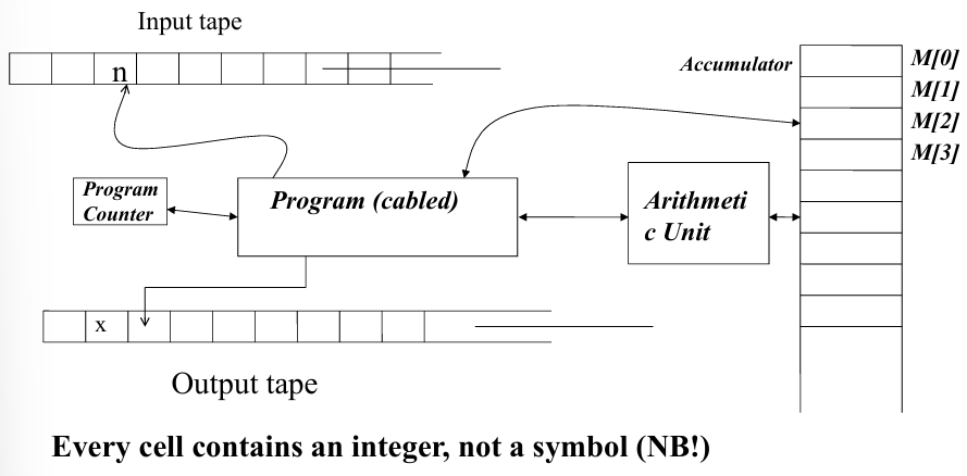
The RAM Machine
The RAM machine is a simple abstract computational model used to describe how certain algorithms are executed on a theoretical machine. It is essential to understand the basic instruction set of the RAM machine to explore its potential in computing tasks. The RAM machine uses a set of instructions to manipulate data stored in memory, perform arithmetic operations, and control the flow of the program. These instructions are categorized into different addressing modes, such as direct, immediate, and indirect addressing.
The RAM machine’s instruction set includes a variety of commands that perform fundamental tasks:
LOAD X M[0] := M[X] % Direct addressingLOAD= X M[0] := X % Immediate addressingLOAD* X M[0] := M[M[X]] % Indirect addressingSTORE [*] X M[X] := M[0], …ADD … M[0] := M[0]+M[X], …SUB, MULT, DIVREAD [*] XWRITE [=, *] X JUMP lab PC := b(lab)JZ, JGZ, ... lab jump if M[0] = 0, > 0, ...HALT
Example
Let’s consider a simple example of a RAM program that computes whether a number is prime. The program reads an input value for , checks if it is divisible by any number between and , and outputs if it is prime, or otherwise.
The RAM program for checking if a number is prime works as follows:
Initialization: The program starts by reading the input value and stores it in memory location . It then checks if equals , as is not a prime number.
Counter Setup: A counter () is initialized to 2, and the program enters a loop where it checks divisibility.
Divisibility Check: For each value of the counter , the program checks if is divisible by . If a divisor is found, is not prime.
Looping: If no divisor is found, the counter is incremented, and the program continues to check divisibility with the next number.
Termination: The loop terminates once the counter exceeds . If no divisors were found, is prime, and the program outputs . Otherwise, it outputs .
The specific assembly code for this program is as follows:
READ 1 % The input value n is stored in cell M[1] LOAD= 1 % If n = 1, it is trivially prime ... SUB 1 JZ YES LOAD= 2 % the counter in M[2] is initialized to 2 STORE 2LOOP: LOAD 1 % If M [1] = M[2] (i.e., counter = n) then n % is prime SUB 2 JZ YES LOAD 1 % If M [1] = (M[1] DIV M[2] ) * M[2] then M[2] % is a divisor of M[1]; hence M[1] is not prime DIV 2 MULT 2 SUB 1 JZ NO LOAD 2 % the counter in M[2] is incremented by 1 and % the loop is repeated ADD= 1 STORE 2 JUMP LOOPYES WRITE= 1 HALTNO WRITE= 0
The execution cost of the RAM program depends on the size of the input .
Space Complexity (): The space complexity of the program is constant, i.e., , because the number of memory locations used by the program does not depend on. The program uses a fixed number of memory cells, regardless of the input size. Specifically, the memory cells for storing , the counter, and some temporary values are the only ones needed.
Time Complexity (): The time complexity of the program is determined by the number of iterations of the loop. The loop runs until the counter reaches , meaning that the program performs iterations (since it starts at 2). Therefore, the time complexity is proportional to , i.e., .
However, it is important to note that this time complexity refers to the number of iterations of the loop, not the length of the input string. The input size is constant because the number is treated as a single integer.
In terms of other algorithms:
Accepting strings like : For algorithms that accept strings and check for specific patterns (e.g., the language ), the space and time complexities are both proportional to the length of the string, i.e., . This means that both the space and time required scale linearly with the input length.
Binary Search: When performing a binary search on a sorted set of numbers, the time complexity is logarithmic, i.e., , assuming the data is stored in memory and the search space is halved with each step.
Sorting Algorithms: The time complexity of sorting depends on the algorithm used. For example, quicksort has an average-case time complexity of .
Complexity Costs Criteria in RAM Machines
When analyzing the complexity of algorithms on RAM machines, we consider two main cost criteria: constant cost model and logarithmic cost model.
In the constant cost model is assumed that every elementary operation—such as an assignment, an arithmetic operation, or a comparison—requires a uniform amount of execution time, irrespective of the data values involved. This approach posits that the time to access a single memory cell or execute a basic instruction is a constant, typically considered to be one unit. This abstract framework is widely used in algorithm theory to simplify asymptotic analysis, allowing us to focus on the growth of the number of operations as a function of the input size, without getting bogged down by the specific details of hardware or implementation.
For instance, within the constant cost model, adding two integers, regardless of their magnitude, always incurs a cost of 1.
In contrast, the logarithmic cost model offers a more realistic representation of the complexity of certain operations, particularly in scenarios where the data can take on very large values. This model is based on the premise that the cost of an operation is not fixed but depends on the size of the data, specifically the length of its binary representation. For an integer , its representation requires approximately bits. Consequently, operations like memory access or calculations on large numbers are modeled with a cost that grows logarithmically with the value of the number itself.
Example
A prime example of this abstraction is the decoding of a memory address; the act of accessing the cell at position may have a cost proportional to because it is necessary to decode an address that is represented by a number of bits proportional to the logarithm of its magnitude.
Aspect
Constant Cost Model
Logarithmic Cost Model
Core Principle
Every elementary operation has a uniform cost of 1, regardless of data size.
The cost of an operation depends on the binary length of the data.
Precision
An abstract simplification, useful for theoretical analysis.
A more realistic model that accounts for data size.
Primary Use
Theoretical algorithm analysis and scenarios with small, fixed-size data.
Analysis of algorithms dealing with very large inputs (e.g., big integer arithmetic, cryptography).
Effect on Time
Execution time remains constant as the data size increases.
Execution time grows logarithmically with the data size.
Computing Using a RAM Machine
Let’s analyze the following C program that computes , which involves repeatedly squaring the number 2:
read(n);x = 2;for (i = 1; i <= n; i++) x = x * x;write(x);
This program starts by reading an integer , initializes a variable to 2, and then iteratively squares for iterations. The result is , as the squaring operation doubles the exponent at each step. However, there’s an important issue when considering the time complexity of this program.
At first glance, the time complexity of this program might seem to be because the loop runs times, and each iteration performs a single arithmetic operation (multiplication). However, this analysis is misleading when we consider the size of the numbers involved.
In each iteration, the value of grows exponentially. On the th iteration, becomes , and after iterations, . The value of after iterations is extremely large, and the number of bits required to represent this value grows exponentially as well.
For instance, the number requires approximately bits to store, as is a number that has binary digits. Hence, the total cost of performing a multiplication operation, which involves manipulating numbers with sizes growing exponentially, is not constant. In fact, each multiplication operation takes time proportional to the number of bits in the numbers being multiplied, which increases rapidly.
Thus, while the program runs iterations, the cost of each iteration is not constant due to the growing size of the numbers involved.
To more accurately analyze the complexity, we need to consider the bit-size of the numbers involved. Specifically:
Time Complexity per Iteration: Each multiplication in the loop involves numbers that grow exponentially in size. The number of bits required to store after iterations is approximately . Multiplying two numbers of bit-length requires time proportional to bits. Therefore, the time to perform the th multiplication is .
Total Time Complexity: The total time complexity of the program is the sum of the time taken for each iteration. If the time for the th iteration is , then the total time complexity is: Hence, the total time complexity is , which is much larger than .
The RAM Model and Precision
The reason this analysis differs from the initial assumption is rooted in the abstract nature of the RAM model. The RAM machine assumes that operations on numbers are unit-cost, meaning each arithmetic operation takes a constant amount of time regardless of the size of the numbers involved. This assumption is valid for small numbers that can be represented within the fixed-width word size of the machine (e.g., 32-bit or 64-bit integers). However, as the numbers grow larger (as they do in this case), this assumption breaks down.
For large numbers, the time required for arithmetic operations scales with the number of bits in the numbers. Therefore, the RAM model is overly simplistic when dealing with operations on large integers like . To handle such numbers, we would need to account for the bit-length of the numbers being operated on, and this would increase the time complexity significantly.
In reality, modern computers work with finite precision.
Example
For example, a 64-bit machine can only store integers up to , and operations on numbers larger than this require special handling, such as using multiple-precision arithmetic.
As the size of the numbers grows (like in this case with ), the time required to store and perform arithmetic on them grows, making the abstract RAM model less practical for such cases.
This is where the issue with the complexity analysis arises: the RAM model does not account for the fact that storing and manipulating large numbers is not a constant-time operation.
Revising the Complexity Based on Bit-Level Precision
A more realistic approach to analyzing this problem involves considering the number of bits required to represent the numbers involved and the cost of operations based on this bit-size. For example, instead of assuming constant-time arithmetic operations, we would analyze the number of bits needed to store and manipulate , and the corresponding cost of each operation.
For large numbers, the complexity of multiplying two numbers of bit-length is (using standard algorithms), and the bit-length grows exponentially as . Thus, a more accurate time complexity for the program would reflect the exponential growth of the number size, leading to a time complexity of , not .
It's also important to note that different computational models may lead to different complexity analyses.
For example, the complexity of an algorithm might vary depending on whether it’s run on a RAM machine, a Turing machine, or a machine with specific hardware optimizations for large numbers (e.g., using multiple-precision arithmetic).
This highlights that the complexity of a problem is not always the same across different models of computation, and the analysis must be adapted to the capabilities and limitations of the model in question.
The Polynomial Correlation Theorem and Its Impact
The Polynomial Correlation Theorem offers a way to relate the complexities of different computation models. This theorem states that
Theorem
If a problem can be solved by a computation model with complexity , then there exists a polynomial such that the same problem can be solved by another computation model with complexity .
This allows us to compare the efficiency of different models and understand their relative strengths and weaknesses, but it also emphasizes that no single model is superior in all cases.
The theorem suggests that
Problems solvable in polynomial time or space on one computational model can also be solved in polynomial time or space on another model, with the complexity being related by a polynomial function.
While a polynomial function can be as large as , it is still much more manageable than exponential growth. For example, compare (where is a constant) to (exponential growth). As grows large, increases much slower than . This is why problems with polynomial complexity, even those with very large exponents like , are still considered “tractable” compared to those with exponential complexity.
Thanks to the Polynomial Correlation Theorem, we can classify problems that are solvable in polynomial time/space as belonging to the class . This class includes problems with complexities like , which are better than exponential ones, but it is also practical in the sense that most real-world problems (such as search problems, pathfinding, and optimization) in typically have manageable degrees (exponents) in their polynomial complexities.
This result ensures that the class of problems solvable in polynomial time/space is invariant across different computational models. In other words, whether we are using a RAM machine or a Turing machine, if a problem is solvable in polynomial time on one, it will also be solvable in polynomial time on the other, even if the exact constants and coefficients might differ.
The analogy of class as “practically tractable” problems reflects that problems solvable in polynomial time are considered feasible for real-world computation. In practice, even problems with high-degree polynomials (like ) can be solved, but problems with exponential growth in complexity (like ) quickly become infeasible as increases.
Simulating a k-Tape Turing Machine with RAM
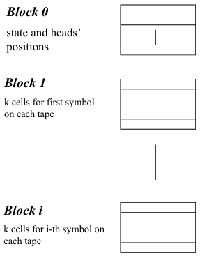
Now, let’s move to the time correlation between a -based model and a RAM-based model. One of the important results here is how a RAM machine can simulate a -tape Turing machine. The RAM memory can simulate the tape by associating each tape cell with a RAM cell. However, instead of allocating blocks of adjacent RAM memory cells for each tape, the simulation works as follows:
Block of Cells for Each Tape: For each -tuple of tape cells, we associate a block of RAM cells. This allows the RAM machine to mimic the structure of the multiple tapes used by the Turing machine.
Base Block: In addition to these blocks, a special “base” block is used to represent the position of the tape head, keeping track of the current state of the machine as it operates.
This approach allows the RAM machine to simulate a Turing machine with multiple tapes, and while the overhead might increase due to the structure of the simulation, the important point is that the simulation is still feasible in polynomial time.
The simulation of Turing machine moves on RAM, and vice versa, highlights the differences in the operational models of these two computational frameworks.
While a RAM machine can simulate a Turing machine with a time complexity proportional to under a constant cost model, more realistic cost models that include logarithmic factors show that the simulation is more complex, involving a complexity.
Conversely, simulating a RAM machine on a Turing machine involves translating each RAM operation into multiple steps on the Turing machine, which often results in higher time complexity compared to the direct execution on the RAM machine.
1. Simulating a Turing Machine Move in RAM
A single move of a Turing Machine (TM) is simulated by a RAM machine, and this involves several operations:
Reading:
The content of a special “0 block” (which holds the state of the machine and possibly other control information) is checked. This requires a sequence of accesses to the memory, where is the number of tapes of the Turing machine. These accesses cost is , where is a constant that accounts for the number of individual operations needed to fetch the necessary information.
To examine the contents of the cells corresponding to the tape heads, indirect accesses are made to the respective blocks in memory. These accesses fetch the values that are currently pointed to by the Turing machine’s heads.
Writing:
The state of the Turing machine is updated. This change is reflected in the “0 block” (which keeps track of the machine’s state).
The values in the RAM corresponding to the cells pointed to by the heads are updated using indirect STORE operations. These operations update the values in the memory, essentially performing the write action of the Turing machine’s tape.
Finally, the positions of the tape heads are updated in the “0 block,” indicating where the heads will move in the next step.
Time Complexity of a Turing Machine Move on RAM
Constant Cost Criterion:
When assuming a constant cost per operation, the total number of RAM moves required to simulate a single move of the Turing Machine is , where is a constant that represents the number of operations needed to handle each read and write action, and is the number of tapes of the Turing Machine. Therefore, the time complexity in this case is
meaning that the time required to simulate the Turing Machine’s move is proportional to the time complexity of the original Turing Machine model.
Logarithmic Cost Criterion:
Under a more realistic cost model, where indirect accesses take logarithmic time (due to the increasing size of the memory addresses as the number of RAM cells grows), the time complexity becomes
where, indicates that the complexity is bounded by a function proportional to . This arises because accessing a particular position in memory requires logarithmic time in the size of the address, and the time complexity is influenced by both the Turing Machine’s complexity and the logarithmic cost of addressing memory positions.
2. Simulating RAM Steps with a Turing Machine
In the context of simulating RAM operations with a Turing Machine (TM), each step in the RAM machine can be broken down into a series of operations that must be translated into Turing machine steps. We will discuss how basic RAM instructions such as LOAD, STORE, and ADD* are simulated on a Turing Machine.
Simulating the LOAD Operation: The RAM instruction LOAD h fetches the value stored at memory location and copies it into the accumulator .
Turing Machine Simulation: The Turing machine must:
Search the tape for the value of . If is not found, this is considered an error.
Once is located, the value is copied onto the tape used for , the accumulator tape. This step requires scanning and copying the relevant part of the tape where the value is stored.
Simulating the STORE Operation: The RAM instruction STORE h writes the value from (the accumulator) to memory location .
Turing Machine Simulation:
The Turing machine must first locate the tape position .
If does not exist on the tape, the Turing machine must “make a hole” (allocate new space) using the service tape and store the value in the appropriate part of the tape that corresponds to .
If already exists, the Turing machine updates the value of by copying into the correct position. This may involve the use of the service tape if the number of cells already occupied by is not the same as the length of .
The process of searching for , copying to , and managing memory allocation with the service tape increases the complexity of this operation on a Turing machine.
Simulating the ADD* Operation: This operation in RAM is responsible for performing addition on the value stored at and updating (the accumulator).
Turing Machine Simulation:
The Turing machine must first locate and fetch the value .
Then, the Turing machine performs the addition operation between the contents of and , storing the result in .
This step involves reading and writing to multiple parts of the tape, similar to the LOAD and STORE operations, but with additional arithmetic steps.
Each RAM move (such as LOAD, STORE, or ADD*) requires multiple operations on the Turing machine’s tapes. Specifically:
Each memory cell in RAM requires multiple tape cells on the Turing machine to represent its content and its address.
For each th RAM cell, the Turing machine needs to store both the address and the value , requiring at least tape cells per memory cell. Additionally, the “service tape” may be used for managing the memory.
Time Complexity of Simulating RAM with Turing Machine
Simulating a RAM machine on a Turing machine involves several complexities:
Each operation on the RAM (such as reading or writing to a memory cell) is translated into multiple operations on the Turing machine’s tapes. These operations involve scanning the tapes and updating values, which typically requires more steps than a simple direct memory access on the RAM machine.
The exact time complexity of this simulation depends on how efficiently the Turing machine can access and update the RAM cells, but generally, it will be higher than the direct simulation of a Turing machine on RAM due to the nature of tape-based memory and the need for sequential access.
Lemma and Time Complexity
Lemma
The length of the Turing machine’s tape, which simulates the RAM, has an upper bound that is proportional to the time complexity of the RAM operation:
The Turing machine requires a time proportional to , where is the time complexity of the RAM operation. The reason for this is that each STORE operation in RAM, which involves updating a memory cell, requires time proportional to the length of the address and the content of the memory cell, both of which must be encoded in the Turing machine’s tape.
For a RAM that performs operations on cells, the total time for simulating this on the Turing machine is proportional to:
where is the length of the address and is the length of the data stored at that address. This sum gives the total time complexity of simulating RAM STORE operations on the Turing machine.
The time required by the Turing machine to simulate a RAM move is at most proportional to , where is the time complexity of the RAM operation. If the RAM move has a time complexity , then the Turing machine can simulate this move in time.
However, the total time to simulate the entire RAM operation on a Turing machine may increase due to the tape management and encoding involved. In the worst case, simulating a RAM with time complexity on a Turing machine requires time. This is because each memory cell involves multiple operations on the Turing machine’s tape, and each operation may depend on the addresses and values being manipulated.
Remarks and Concluding Warnings
When discussing time complexity and computational models, it is important to consider the data dimension parameter. This refers to various aspects of the data, which can affect the overall complexity of the problem:
Input String Length: The size of the input string or data representation.
Value of the Datum (): The magnitude or size of individual data values, such as in algorithms that operate on numbers.
Number of Elements: The size of data structures, like the number of nodes in a graph, rows in a matrix, or elements in a table.
These parameters are often related, but they are not always linearly correlated. For instance, the value often requires an input string of size . This means that when analyzing complexity, it is essential to distinguish between the physical size of the input (number of bits required to represent the data) and the logical size of the data (the number of elements or entities being manipulated).
Binary Search and Polynomial Correlation Theorem
A key question to consider is whether an algorithm like binary search, when implemented on a Turing machine, violates the Polynomial Correlation Theorem. Binary search has a time complexity of when searching in a sorted list of size . On a Turing machine, however, it would require additional steps due to the sequential nature of tape access and would likely result in an overall time complexity of .
At first glance, it might seem like this violates the polynomial correlation theorem. However, this is not necessarily the case. The theorem applies to the general transformation of complexity across different computational models, but it assumes reasonable conditions about memory access and other factors, such as whether data is already in memory.
For a Turing machine, it is important to recognize that data is not assumed to be in memory in the same way it is in a RAM machine, which has direct access to memory cells. In practical terms, this results in at least linear complexity for data access (since searching the tape is a linear operation), making the analysis more complex.
Thus, the linear overhead added by Turing machine tape operations in the case of binary search does not violate the polynomial correlation theorem. Rather, it reflects the inherent inefficiency of simulating a RAM-like operation with a Turing machine.
Average Case vs. Worst Case Complexity
While average-case performance is often used in practice (e.g., for algorithms like Quicksort or during compilation), this approach is not suitable for all scenarios, particularly in critical or real-time applications. In these cases, worst-case complexity is of much greater importance because the algorithm needs to handle the most extreme inputs in a predictable manner. Real-time applications, such as those used in embedded systems or safety-critical applications, cannot rely on average-case behavior due to the unpredictability of inputs.
Therefore, it is crucial to carefully assess the computational models and algorithms used in such scenarios to ensure that the performance remains within acceptable bounds, even in the worst case.