2.3 - Turing Machine

---

️️️The Turing Machine is an historical model of a “computer”, simple and conceptually important under many aspects. We consider it as an automaton; then we will derive from it some important, universal properties of automatic computation. For now we consider the -tape version, slightly different from the (even simpler) original model.

k-tape Turing Machine

The -tape Turing Machine represents an advanced configuration of the classical Turing Machine, which is essential for understanding various aspects of computation. In this model, the operational structure remains similar to that of other automata, with consistent states and alphabets defining the input, output, control device, and memory alphabet. This version introduces multiple tapes (specifically tapes) each serving as a distinct medium for reading and writing symbols, thereby enhancing the machine’s computational capabilities.

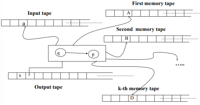
Historically, Turing Machines have been depicted with infinite sequences of cells labeled as , as opposed to finite strings. This choice stems from certain mathematical considerations that facilitate more comprehensive analyses of the machine’s functionality. Each tape in a -tape Turing Machine is assumed to contain a finite number of non-blank symbols, with the remainder of the tape filled with a designated “blank” symbol, often represented as ” ” (empty space) or . The decision to model the tapes as infinite sequences allows for a more elegant mathematical treatment of the Turing Machine, as it simplifies the representation of states and transitions.

Each of the tapes operates independently, with the first tape frequently designated to contain a special symbol, , which plays a crucial role similar to the initial state in other computational models, such as the Pushdown Automaton (PDA). This special symbol serves as a marker for the machine’s operational context and aids in the organization of data across the multiple tapes.

Furthermore, the -tape Turing Machine includes scanning heads for both input and output, mirroring the functionality of previous models. These heads are capable of reading symbols from the tapes and writing new symbols based on the current state of the machine. The parallel access to multiple tapes significantly increases the efficiency of data processing, as it allows the machine to perform several operations simultaneously. This characteristic is particularly advantageous for tasks involving complex computations or those that would require extensive sequential processing in a single-tape setup.

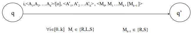
The Movements of the Turing Machine

The movement of a Turing Machine, specifically in the context of a -tape machine, is dictated by the interaction between its internal state, the input tape, the memory tapes, and its control device. At each step of computation, the machine reads one symbol from the input tape and symbols, one from each of the memory tapes. Additionally, it considers the current state of its control device to determine the subsequent actions. These actions can be categorized as follows:

1. State Transition: The control device transitions from one state to another state . This represents the internal computation logic that determines the next step based on the machine’s current configuration.
2. Writing on Memory Tapes: For each memory tape (where ), the machine writes a new symbol in place of the symbol that was just read. This action updates the memory content of the machine.
3. Writing on the Output Tape: If required, the machine can also write a symbol on the output tape. This symbol is typically used to store results or intermediate outputs of the computation.
4. Moving the Heads: The machine moves its reading and writing heads across the tapes. Specifically:
   • The memory tape heads (one for each of the tapes) and the input tape head can move one position to the right (denoted as ), one position to the left (denoted as ), or stay in the current position (denoted as ).
   • The output tape head, however, can only move right or stay in place, as output typically follows a sequential pattern.

Thus, the machine’s configuration evolves through a combination of state transitions, writing symbols, and head movements. This can be formalized using a transition function, , which governs how the machine moves from one configuration to the next.

Definition

The formal structure of this transition is:

In this expression:

• represents the set of states of the control device.
• denotes the input alphabet.
• is the memory alphabet (symbols written on the memory tapes).
• is the output alphabet (symbols written on the output tape).

The function describes the machine’s transition by determining the new state, the symbols to be written on the memory tapes, and the directions in which the heads will move.

When the Turing Machine begins its computation, the system is initialized as follows:

• The memory tapes contain a special starting symbol followed by an infinite sequence of blank symbols.
• The output tape is initially blank.
• The heads of all tapes (input, memory, and output) are positioned at the 0^th cell.
• The control device is set to its initial state .
• The input string is placed on the input tape starting from the 0^th position, followed by blanks.

The machine halts when it reaches an accepting state, denoted by , which is a subset of all possible states. The formal convention is that when the machine reaches an accepting state , the transition function no longer produces any action. In other words, once the machine is in an accepting state, it stops, and no further transitions occur. The machine accepts the input string if it halts after a finite number of moves and its final state belongs to .

Formalization of Transitions (for k = 1)

To simplify, consider a 1-tape Turing Machine.

Definition

The transition between configurations is formalized as:

In this notation:

• are the current and next states.
• is the current input symbol being read.
• represent the portions of the input tape to the left and right of the read symbol.
• represent the portions of the memory tape to the left and right of the current symbol.
• is the symbol currently being read on the memory tape.

The transition function for this 1-tape machine takes the current state , the input symbol , and the memory symbol and produces a new state , a new memory symbol , and movement instructions and for the input and memory heads, respectively.

• If , the input head stays in place, and and remain unchanged.
• If , the input head moves right, appending to , and if is empty, it is replaced with a blank symbol.
• If , the input head moves left, and the tape contents are adjusted accordingly.

The movement for the memory head follows similar rules, adjusting the position of the head on the memory tape.

• If , the memory symbol remains unchanged, and the tape contents are updated accordingly.
• If , the memory symbol is replaced by , and if the right portion of the tape is empty, it is filled with a blank symbol.
• If , the memory symbol is replaced by , and the tape contents are adjusted accordingly.

Language of a Turing Machine

In formal language theory, a Turing Machine defines a language by determining whether a string is accepted by the machine. A string is accepted by the TM if, starting from an initial configuration, the machine halts in an accepting state after a series of transitions.

Given the initial configuration:

where:

• is the initial state,
• is the input string, and
• is the special symbol on the memory tape that marks the beginning of the computation

The machine processes the input, transitioning through a series of configurations until it reaches the final configuration :

where:

• is an accepting state from the set of final states ,
• represents the processed input on the input tape,
• represents the contents of the memory tape at the time the machine halts.

The symbol represents the sequence of transitions leading from the initial configuration to the final configuration, and the machine halts if there is no further configuration to transition to, i.e., .

Thus, the language of the Turing Machine , denoted , is the set of all strings (where is the input alphabet) that are accepted by the machine:

A string is not accepted by the Turing Machine if one of the following conditions holds:

1. Halt in a Non-Accepting State: The TM halts in a state , meaning the machine has reached a state that is not part of the set of final accepting states.
2. Non-Halting (Infinite Loop): The TM never halts, which is an important case in the theory of computation. If the machine continues indefinitely without reaching a halting configuration, the input is not accepted. This case highlights one of the significant challenges in computation—deciding whether a machine will halt on a given input.

Similarity to Pushdown Automaton

The Turing Machine shares similarities with the Pushdown Automaton (PDA), specifically in the case where the PDA may not accept an input due to a “non-stopping run,” meaning the PDA does not halt. However, a critical question in theoretical computer science is whether there exists a loop-free Turing Machine, a machine that always halts regardless of the input. This leads into deeper exploration of decidability and the halting problem, which proves that no general algorithm can determine whether a Turing Machine halts for every possible input.

Example: Turing Machine for

Consider a Turing Machine that accepts the language , where the machine must process an equal number of as, bs, and cs in that order. The machine operates as follows:

1. It starts in an initial state and scans the input tape for an a.
2. Once it finds an a, it marks it and moves to state , where it scans for a corresponding b.
3. After finding a b, it marks it and moves to state , where it scans for a corresponding c.
4. After processing a c, it moves to state , checks for more input, and repeats the process if necessary.
5. Finally, when all as, bs, and cs are processed, the machine moves to the accepting state .

The machine’s behavior can be visualized with the following state transitions:

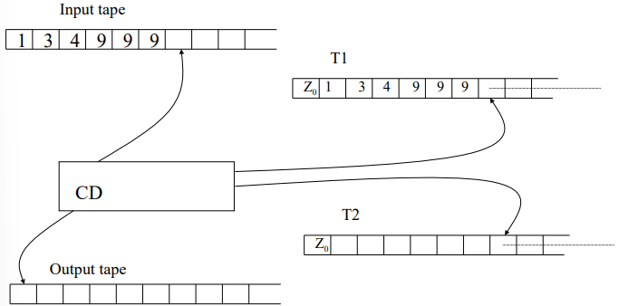
Example: Computing the Successor of a Number

Another example of a Turing Machine’s computational power is a machine that computes the successor of a number , encoded in decimal digits. The machine uses two memory tapes ( and ) to perform the computation:

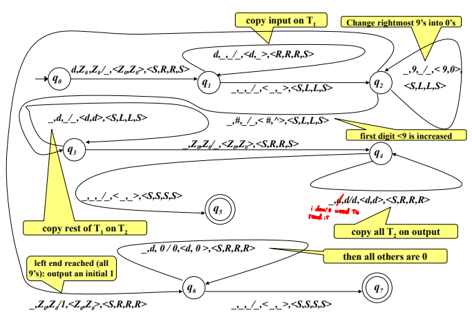
6. The machine copies the digits of from the input onto tape , to the right of the special symbol . Simultaneously, the head on tape moves to the corresponding position.
7. The machine then scans the digits on from right to left, changing the digits as needed. For example, digits equal to 9 are turned into 0, and the first digit not equal to 9 is incremented by 1. All digits to the left of this first non-9 digit remain unchanged.
8. The updated number is copied from to the output tape.

The key symbols used in this process are:

Symbol	Meaning
d	Any decimal digit
_	Blank
#	Any digit not equal to 9
^	Successor of a digit denoted as # (in the same transition)

Closure Properties of Turing Machines

The closure properties of Turing Machines are an important aspect of understanding the computational power of these abstract machines. These properties describe the behavior of Turing Machines under various operations on languages, such as intersection, union, and concatenation.

For intersection, denoted by , Turing Machines are closed under this operation.

This means that, given two Turing Machines and , there exists another Turing Machine that accepts the language that is the intersection of the languages accepted by and .

Intuitively, a Turing Machine can simulate two other TMs either “in series” or “in parallel,” depending on the specific construction of the simulation. For example, a Turing Machine could interleave the steps of and , running them concurrently, and only accept the input if both machines do. Therefore, the intersection operation is easily handled by Turing Machines.

Similarly, Turing Machines are closed under union (), concatenation, and the Kleene star operation (). In each case, Turing Machines can be constructed to simulate the necessary combinations of inputs and transitions to perform the operations on the languages.

Complementation of Turing Machines

However, when it comes to complementation, the situation is more complex. The complement of a language accepted by a Turing Machine would consist of all strings that are not accepted by the machine. However, Turing Machines are not closed under complementation. This negative result arises from the fact that Turing Machines do not always halt—there may be cases where the machine runs indefinitely without reaching a final state.

If there existed a class of loop-free Turing Machines, i.e., machines that always halt regardless of the input, complementation would be straightforward. In this case, one could simply define the set of halting states and partition them into accepting and non-accepting states. By ensuring that halting states are disjoint from non-halting states, it would be possible to construct a Turing Machine that complements any language. However, since Turing Machines may enter non-terminating computations (i.e., infinite loops), it is impossible to define a general method to complement a language without addressing the issue of non-halting computations. This highlights one of the central limitations of Turing Machines.

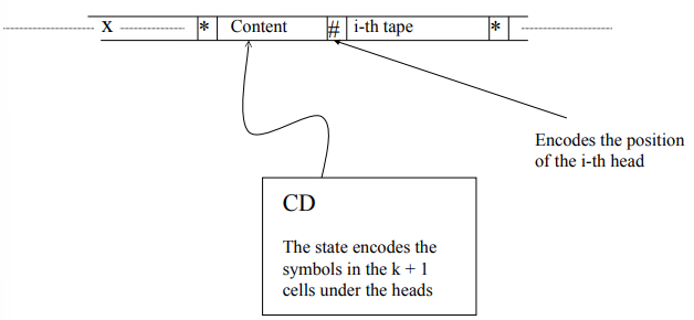
Universal Turing Machine

A Universal Turing Machine (UTM) is a special type of Turing Machine that can simulate any other Turing Machine. A key concept in the theory of computation, the UTM essentially embodies the idea of a general-purpose computer capable of running any algorithm provided as input. In contrast to specific Turing Machines designed to solve particular problems, the Universal Turing Machine takes as input a description of another Turing Machine (encoded as a string) along with the input for that machine. It then simulates the behavior of on .

The UTM can be described as a single-tape Turing Machine, where the single tape serves multiple roles:

• Input: The machine receives the encoding of both the target machine and the input to simulate.
• Memory: The same tape is used to store intermediate results and configurations during the computation.
• Output: Once the computation is complete, the result of the simulation is also written on the same tape.

It is important to note that a single-tape Turing Machine is distinct from a Turing Machine with only one memory tape.

In the single-tape UTM, the input, memory, and output all occupy the same physical tape, while a standard multi-tape TM may have separate tapes for input, memory, and output.

Despite this distinction, all versions of Turing Machines are equivalent in terms of their computational power. In other words, regardless of how many tapes a Turing Machine uses, it can solve the same class of problems.

Turing Machines and Von Neumann Architecture

One of the fascinating aspects of the Universal Turing Machine is its relation to more “realistic” computing models, such as the Von Neumann architecture, which is the foundation for most modern computers. While the Turing Machine is an abstract model of computation, the Von Neumann machine is a concrete model of actual physical computers. Despite these differences, a Turing Machine can simulate a Von Neumann machine.

The primary distinction between the two models lies in the way they access memory:

• A Turing Machine accesses memory sequentially, moving its head one cell at a time.
• A Von Neumann machine, on the other hand, accesses memory in a random-access manner, allowing it to directly retrieve any memory location without sequential traversal.

This difference in memory access does not affect the computational power of the two models; both are capable of solving the same class of problems (i.e., both are Turing complete). However, it does influence the efficiency of computation. In particular, the time and space complexity of certain algorithms may differ significantly between a Turing Machine and a Von Neumann machine due to the different memory access methods. While Turing Machines are theoretically powerful, the sequential nature of memory access can lead to inefficiencies, especially for problems that benefit from random-access memory.

In the context of complexity theory, this distinction between memory access methods becomes important, as it affects the amount of time and memory required to solve a given problem. Therefore, while Turing Machines provide a fundamental model for understanding computation, the practical implications of computational complexity must consider factors such as memory access patterns and machine architecture.