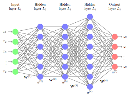
A Feedforward Neural Network (FFNN) is a type of artificial neural network characterized by its structure and flow of information. Here are the key aspects of FFNNs:
- Feedforward Structure: Information flows unidirectionally from the input layer to the output layer, with no feedback loops or cycles in the network. This acyclic nature ensures that inputs are processed in a straightforward manner without revisiting previous layers.
- Layered Architecture: FFNNs are composed of multiple layers of neurons, including one or more hidden layers. Each layer contains neurons that apply an activation function to their inputs, transforming the data as it passes through the network.
- Connections Between Layers: Every neuron in a layer is connected to all neurons in the subsequent layer, creating a dense network of connections. However, neurons in the same layer do not connect to each other.
- Weight Definitions: The connections between neurons are represented by weights
, where: is the layer index, is the neuron index in layer , is the neuron index in layer .
The output of each neuron in a given layer depends on the outputs of the previous layer, defined mathematically as:
The total number of weights in an FFNN can be calculated as
is the number of neurons in the input layer, is the number of neurons in the hidden layer, - The
accounts for the bias term.
This indicates that the number of weights grows quadratically with the number of neurons in the hidden layer.
Universal Function Approximation
One of the most significant properties of FFNNs is their capability as universal function approximators. This means they can approximate any continuous function given enough neurons in the hidden layer. The non-linearity introduced by the activation functions is crucial, as it allows the network to capture complex relationships between inputs and outputs.
“A single hidden layer feedforward neural network with
-shaped activation functions can approximate any measurable function to any desired degree of accuracy on a compact set.”
This theorem implies that even a single hidden layer can represent any function. However, this does not guarantee that a learning algorithm can efficiently find the necessary weights to achieve this approximation. In the worst case, an exponential number of hidden units may be required, making the network impractical. Furthermore, a large number of hidden neurons could lead to difficulties in learning and generalization, causing overfitting to the training data.
Activation Functions in Neural Networks
The activation function of a neuron determines the output based on its input. It introduces non-linearity, enabling the neural network to learn complex patterns. Here are some of the most commonly used activation functions:
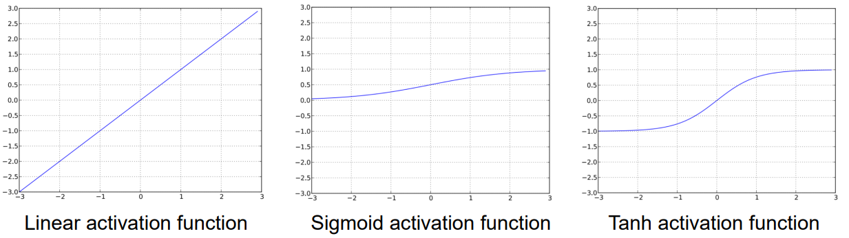
| Linear Activation Function | Sigmoid Function | Hyperbolic Tangent (Tanh) Function | |
|---|---|---|---|
| Definition | |||
| Derivative | |||
| Use Case | Often used in the output layer for regression problems, where the network predicts continuous values over | Commonly used in the output layer of binary classification problems where the goal is to output a probability between 0 and 1. | Suitable for hidden layers and certain classification tasks where the output classes are |
Warning
For hidden neurons, either the sigmoid or tanh functions are usually preferred. The choice of activation function for the output layer depends on the type of problem being solved.
Activation Functions for Output Layers
-
Binary Classification
- If the two classes are encoded as
, then tanh is a suitable choice. - If the two classes are encoded as
, the sigmoid activation function is used. The sigmoid’s output represents the probability of the input belonging to class 1.
- If the two classes are encoded as
-
Multiclass Classification For problems with more than two classes, each output neuron corresponds to a class, and one-hot encoding is used for the labels. One-hot encoding assigns a unique vector for each class:
In this case, the softmax activation function is applied to the output layer:
Definition
The softmax function is defined as
where
represents the probability of class , is the input to the th neuron in the output layer, and is the total number of classes.
The softmax function converts the raw scores (logits) into probabilities, ensuring that the sum of the probabilities across all classes is equal to 1. This is particularly useful in multiclass classification problems where the goal is to output a probability distribution across multiple classes.
Optimization and Learning in Neural Networks
The task of training a neural network is essentially finding a set of parameters (weights
Given a training set
where
The most common way to measure the error in regression problems is the Sum of Squared Errors (SSE). It calculates the total squared difference between the network’s predictions and the actual target values. Mathematically, it is defined as:
where:
is the error (or loss) function, is the number of data points in the training set, is the actual target value for the th data point, is the predicted output from the network for the th input.
The SSE is a commonly used loss function in regression problems. It works well because it penalizes larger errors more heavily, driving the optimization process toward minimizing significant prediction deviations.
The sum of squared errors (SSE) is a straightforward way to quantify the difference between predicted values and actual target values, especially useful in regression tasks.
Non-linear Optimization
The process of training a neural network can be framed as a non-linear optimization problem, where the objective is to minimize the error function with respect to the weights of the network. However, unlike simple convex problems, neural network error functions are typically non-convex, meaning they have multiple local minima and saddle points. This makes finding the global minimum more challenging.
Gradient Descent for Weight Optimization
To minimize the error function, we use gradient descent. The update rule for gradient descent is based on computing the derivative (gradient) of the error function with respect to the weights and moving in the direction of the negative gradient to reduce the error.
where:
is the weight vector at iteration , is the learning rate, controlling the step size of each update, is the gradient of the error function with respect to the weights.
The learning rate
- If
is too small, the convergence will be slow. - If
is too large, the algorithm may overshoot the minimum and oscillate, possibly diverging.
In neural networks, the error function
To improve convergence and help escape local minima, optimization techniques introduce various modifications, such as momentum.
Definition
Momentum is a technique that helps the gradient descent algorithm escape local minima and speed up convergence. It does this by incorporating information from previous iterations, effectively smoothing out the weight updates.
The update rule with momentum is:
where
Momentum allows the optimizer to “build up speed” in directions of consistent gradients, helping it avoid getting stuck in small local minima or plateaus. A typical value for
To ensure that the optimization algorithm converges to a global minimum, the learning rate is often decreased over time. A common practice is to start with a relatively large learning rate and then reduce it gradually as training progresses. This allows the optimizer to take larger steps initially to explore the solution space and smaller steps later to fine-tune the weights.
Advanced Optimization Algorithms
While gradient descent and momentum work well in many cases, more sophisticated optimization algorithms have been developed to handle the challenges of non-convex optimization more effectively. Some popular algorithms include:
- Adam (Adaptive Moment Estimation): Combines the advantages of both RMSprop and momentum. It computes individual adaptive learning rates for each parameter based on the first and second moments of the gradients.
- RMSprop (Root Mean Square Propagation): Adaptively adjusts the learning rate based on the running average of the squared gradients. It helps in reducing the oscillations and improving convergence speed.
- Adagrad: Adjusts the learning rate for each parameter based on the history of gradients, allowing for larger updates for infrequent features and smaller updates for frequent features.
These advanced algorithms automatically adjust the learning rate during training, which improves the overall optimization process and helps find better configurations of weights.
Example
Consider a neural network with a single hidden layer with an output function defined as
and an error function . We want to compute the weight update for the weight .
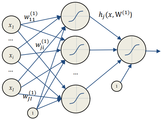
Putting all together, we have
This formula, which use all the samples at the same time (one step, all the data) is called batch learning. It is the most efficient way to learn the weights of a neural network. However, it is not always possible to use all the data at the same time due to memory constraints. In this case, we can use different strategies:
- Batch gradient descent: update the weights using all the samples at the same time
- Stochastic gradient descent: update the weights using one (unbiased) sample at the time with high variance
- Mini-batch gradient descent: update the weights using a subset of the samples at the same time. Good trade-off between the two previous methods
The batch learning algorithm is the most efficient way to learn the weights of a neural network and could be easily computed automatically by the backpropagation algorithm.
Backpropagation and the Chain Rule
The backpropagation algorithm is a fundamental method used in training neural networks, allowing efficient computation of gradients for weight updates. It leverages the chain rule of calculus, which facilitates the calculation of the derivative of composite functions. Here’s how it works:
Definition
The chain rule states that if you have a composed function
, the derivative of with respect to can be computed as follows:
where:
identifies the intermediate variable between and . is the derivative of evaluated at is the derivative of evaluated at
This principle applies directly to the backpropagation process in neural networks.
During backpropagation, we compute the gradient of the error function with respect to each weight in the network, propagating the error backward through the layers. The general update rule can be derived using the chain rule.
Given the error function defined as:
the partial derivative of the error function with respect to a weight
Breaking this down, we have:
-
Error term:
This term represents how the output of the network differs from the target value. -
Activation function derivative:
This term is the derivative of the activation function, which describes how the output of a neuron changes with respect to its input. -
Weight influence:
This term indicates how the weighted input changes with respect to the weight . -
Propagation through layers: The update for weights in the preceding layers can also be computed similarly, propagating the gradients back through the network.
While the sum of squared differences works well for regression problems, it may not be the most effective choice for classification tasks. In classification problems, especially when dealing with multi-class classification, we often use the cross-entropy loss function, defined as:
where:
is a binary indicator (0 or 1) that indicates whether class label is the correct classification for observation . is the predicted probability that observation belongs to class .
The cross-entropy loss provides better gradient signals during training, especially for deep networks, leading to improved convergence and performance.
Note on Maximum Likelihood Estimation
Let’s observe indipendent and identically distributed (i.i.d.) samples from a Gaussian distribution with known variance
The probability distribution of the samples is
. The likelihood of the samples is the probability of observing the samples given the parameters of the distribution. The maximum likelihood estimation (MLE) is the method used to estimate the parameters of the distribution that maximize the likelihood of observing the samples. The paramenters estimated using MLE are unbiased and have the minimum variance among all unbiased estimators. To calculate the MLE, we have to follow a simple recipe: let
a vector of parameters:
- Write the likelihood function
for the data
- Take the
of the likelihood function (this step is optional, but it makes the calculations easier since the function is monotonic)
- Work out
(or ) for each parameter
- Solve the set of simultaneous equations
(or ) for the parameters
\end{aligned}$$
- Check that
is a maximum To maximize/minimize the (log)likelihood you can use several techniques, like analytical solutions (solve the equations), numerical solutions (like gradient descent), or optimization algorithms (like Lagrange multipliers).
In case of classification problems, when looking for the weights which maximize the likelihood of the data, we can use the
function
where
is the target value and is the output of the network. The function gives the same weights to all the samples, and the function has the same effect of the function. For classification problems, using SSE as the error function may not be the best choice because the error function depends only on the distribution of the error (and not on the value of the error). Also, the distribution is not Gaussian, but it is a Bernoulli distribution. We have some i.i.d samples coming from a Bernoulli distribution
To calculate the MLE, we have to follow the same steps as before:
Choosing the Error Function
The choice of the error function plays a crucial role in neural network optimization, as it defines what kind of learning the network will perform. Here are key considerations for selecting the appropriate error function:
| Error Function | Sum of Squared Errors (SSE) | Binary Cross-Entropy (BCE) |
|---|---|---|
| Formula | ||
| Use Case | Suitable for regression problems, where the goal is to minimize the difference between the predicted and actual values. The SSE error function is ideal when the output is continuous. | Most suitable for binary classification tasks where the output is either 0 or 1. BCE measures the difference between the predicted probability distribution and the actual binary distribution. |
| Intuition | The SSE error function penalizes large errors more heavily than small ones due to the squaring of the error term, making it useful in cases where you want to avoid large deviations from the target values. | Cross-entropy measures how well the model’s predicted probability distribution matches the true distribution, encouraging outputs that are closer to the target class probabilities. |
| Key Feature | The gradient for SSE is easier to compute for continuous output, making optimization straightforward. | BCE is sensitive to the probability estimates of the network, making it particularly good for probabilistic interpretation, such as predicting class membership probabilities. |
Choosing the error function requires careful consideration of the following:
-
Problem Type:
- Regression: SSE is often the best choice because it aligns well with continuous output ranges.
- Binary Classification: BCE is typically preferred due to its probabilistic interpretation, especially when dealing with outputs between 0 and 1.
- Multi-Class Classification: In cases with more than two classes, categorical cross-entropy (an extension of BCE) is often used.
-
Data Distribution: Exploit any background knowledge on how the data is distributed. For instance, if data follows a Gaussian distribution, SSE might be a natural choice. For other distributions, such as those encountered in classification, cross-entropy is typically a better fit.
-
Task Constraints: The constraints and goals of the task, such as sensitivity to outliers or emphasis on correctly classifying a particular class, can guide the choice of error function.
-
Trial and Error: Often, practitioners experiment with different loss functions and observe how the model behaves. This empirical approach helps fine-tune performance, especially in complex tasks where assumptions about the data distribution may not be entirely correct.
Hyperplane and Linear Algebra
A hyperplane is a flat affine subspace of one dimension less than its ambient space. In machine learning, hyperplanes are used as decision boundaries in classifiers like perceptrons and support vector machines (SVMs).
Definition
A hyperplane in
can be defined as:
where
is the bias term and is the weight vector normal to the plane. For any two points and on , the difference vector lies perpendicular to :
The signed distance from a point
Perceptron Learning Algorithm
The perceptron is a linear classifier that separates data using a hyperplane. Its goal is to find a hyperplane that correctly classifies all training points.
Let the perceptron output be coded as +1 or -1. If a point is misclassified:
- If the correct label is +1 but the output is negative:
- If the correct label is -1 but the output is positive:
The error function for the perceptron minimizes the total distance of misclassified points from the hyperplane:
To minimize this error function, we use stochastic gradient descent (SGD). The gradients with respect to the weight vector
The perceptron learning rule can be seen as a form of Hebbian learning, where the weights are adjusted to reinforce the correct classification of the inputs based on their label.