Artificial Intelligence (AI) represents the expansive field of technology dedicated to enabling machines to replicate human-like intelligence. It encompasses a broad spectrum of techniques and approaches aimed at imbuing machines with capabilities such as reasoning, learning, problem-solving, perception, and language understanding. AI techniques are crucial in enabling computers to perform tasks that traditionally require human cognitive abilities, ranging from simple decision-making processes to complex problem-solving scenarios.
The evolution of AI can be traced back to seminal events like the Dartmouth Conference of 1956, organized by John McCarthy, Marvin Minsky, Nathaniel Rochester, and Claude Shannon. This landmark event laid the foundation for AI research, proposing a focused exploration into how machines could simulate human intelligence. Early AI developments were rooted in the desire to expand computational capabilities beyond the strictly procedural tasks performed by early computers in the 1940s, which were primarily focused on executing predefined instructions and rapid arithmetic operations.
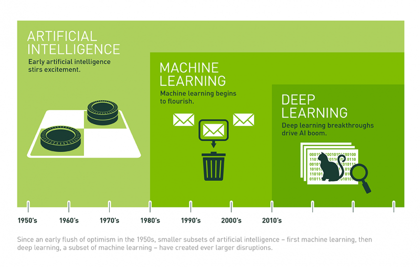
Machine Learning (ML) emerges as a specialized subset within AI, emphasizing the ability of machines to autonomously learn and improve from experience without being explicitly programmed. ML algorithms analyze vast amounts of data to uncover patterns, make predictions, or inform decisions. The process involves data sorting and filtering, which are depicted in the image to illustrate how ML algorithms learn and adapt based on the information they process.
Deep Learning (DL) represents a further refinement within ML, characterized by neural networks with multiple layers (hence “deep”) that enable sophisticated data processing and feature extraction. DL has significantly advanced AI capabilities, particularly from the 2010s onward, leveraging computational resources like cloud computing and complex data analysis represented in the image by icons of cloud networks and binary code. This technological advancement has enabled breakthroughs in tasks such as image and speech recognition, natural language processing, and autonomous systems.
The quest for AI capabilities beyond traditional computing paradigms, such as the Von Neumann architecture, reflects ongoing efforts to create machines that can interact with unstructured data, operate in dynamic environments, and adapt to new circumstances autonomously. This evolution underscores AI’s trajectory from its theoretical origins to its practical applications in modern computing and beyond, driving innovation across various industries and societal domains.
The Brain Computational Model
The human brain, even in the 1950s, was well-documented and studied, serving as the inspiration for computational models that inform the development of artificial neural networks. With an intricate network of neurons and synapses, the brain showcases extraordinary computational capabilities through its distributed, fault-tolerant, and parallel processing nature.
The brain consists of approximately
The brain’s computational model can be broken down into three primary characteristics:
- Distributed Processing: Computation within the brain is distributed across billions of neurons, each contributing to overall cognitive function. Neurons act as non-linear units, meaning their output is not directly proportional to their input, allowing for complex processing capabilities.
- Fault Tolerance: The brain’s architecture is designed to be redundant. If a neuron fails or becomes damaged, other neurons can compensate, ensuring that the system as a whole remains functional. This fault tolerance provides resilience and robustness to brain functions.
- Parallelism: Neuronal computation is inherently parallel. Multiple neurons fire simultaneously, allowing the brain to process numerous pieces of information concurrently. This parallel nature enables the brain to perform complex tasks, such as pattern recognition, decision-making, and motor coordination, with remarkable speed and efficiency.
Definition
A neuron is a highly specialized cell that serves as the building block of the brain and nervous system. Its primary function is to transmit information via electrical and chemical signals. The anatomy of a neuron consists of three main parts: the cell body (soma), dendrites, and an axon. The soma houses the nucleus and organelles, while dendrites are the branch-like extensions that receive incoming signals. The axon is a long fiber responsible for transmitting outgoing signals to other neurons or cells.
Neuronal communication begins when a neuron receives a signal, either from another neuron or external sensory input. This signal causes a change in the electrical charge across the neuron’s membrane, initiating an action potential. The action potential occurs when the neuron’s membrane potential reaches a specific threshold, opening voltage-gated ion channels. As a result, sodium ions (
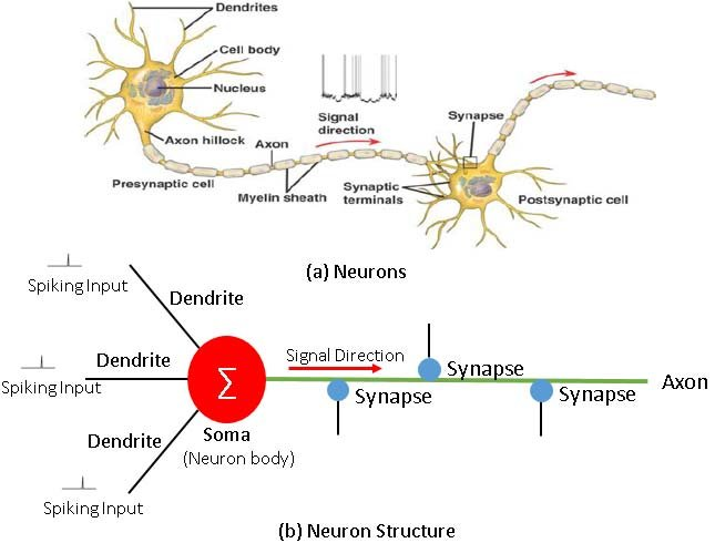
Once the action potential reaches the end of the axon, it triggers the release of neurotransmitters from vesicles within the axon terminals. These neurotransmitters are chemical messengers that are released into the synaptic cleft, a narrow space between the transmitting neuron’s axon terminal and the receiving neuron’s dendrites.
Upon release, neurotransmitters bind to specific receptors on the dendrites of the receiving neuron, causing ion channels to open and allowing ions to flow in. This influx of ions generates a new electrical signal within the receiving neuron, propagating the transmission of information. This process, known as synaptic transmission, is the fundamental mechanism by which neurons communicate and form the intricate networks that drive all brain functions.
The computational model of the brain, with its distributed, fault-tolerant, and parallel processing capabilities, has been a major influence on the development of artificial neural networks, particularly in AI and machine learning. By mimicking the brain’s ability to process information in a distributed and parallel fashion, artificial systems have been designed to perform complex tasks like image recognition, speech processing, and autonomous decision-making.
Computation in Artificial Neurons
In 1943, Warren McCulloch and Walter Pitts introduced one of the first formal models of an artificial neuron, known as the Threshold Logic Unit or Linear Unit. This model used a threshold-based activation function, equivalent to the Heaviside step function, to determine whether or not the neuron “fired” based on input signals.
A significant advancement came in 1957 when Frank Rosenblatt developed the first Perceptron, an early form of neural network used for binary classification tasks. In Rosenblatt’s perceptron, weights were encoded in potentiometers, and electric motors were used to update these weights during the learning process. By 1960, Bernard Widrow introduced the idea of representing the threshold as a bias term in the ADALINE (Adaptive Linear Neuron), further refining the model.
Definition
The Perceptron is a single-layer neural network designed for two-class (binary) classification problems. It processes input signals, computes a weighted sum, and applies an activation function to produce an output. While simple, the perceptron model laid the groundwork for more complex neural networks used today.
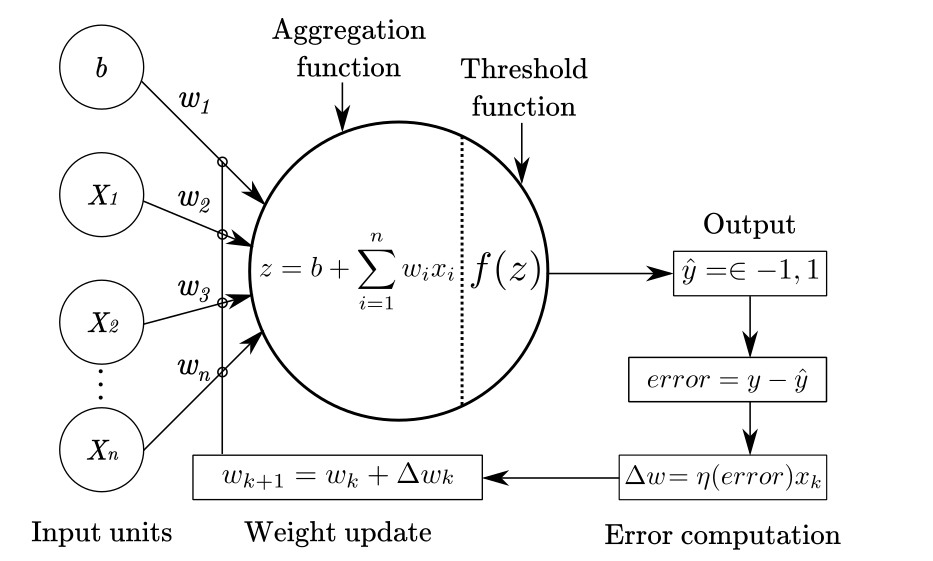
Artificial neurons receive input signals (
- Input Signals (
): These are the data or signals provided to the neuron. - Weights (
): Each input is associated with a weight, which can either be positive (excitatory) or negative (inhibitory). The weight determines the importance of the input. - Accumulator Function (
): This function sums the weighted inputs. - Bias (
): An additional parameter that shifts the activation function’s decision boundary, allowing the neuron to better fit the data. - Activation Function (
): This non-linear function determines the neuron’s output based on the accumulated input. It can be a step function, sign function, sigmoid, ReLU, or other types of activation functions.
The output of the neuron, denoted as
where,
Perceptron Example
Consider a single perceptron with two inputs,
and , and a bias term . The weight vector is , and the activation function is a step function. The output is determined as:
In this case, the perceptron acts as a logical OR gate. The output will be 1 if at least one of the inputs is 1, as shown in the following table:
1 0 0 0 1 0 1 1 1 1 0 1 1 1 1 1 For a different set of weights, say
, we can modify the perceptron to behave like a logical AND gate. The output is calculated as:
This perceptron outputs 1 only when both
and are 1, mimicking the logical AND operation.
The perceptron’s simplicity is its strength and limitation. While it can solve linearly separable problems (like OR or AND logic gates), it struggles with more complex, non-linear problems. This limitation was formally proven in the late 1960s with the XOR problem, where a single-layer perceptron could not solve the problem. However, the introduction of multi-layer perceptrons (MLPs) and the backpropagation algorithm in later years addressed this limitation by allowing deeper, more complex neural networks capable of solving non-linear problems.
Hebbian Learning
In 1949, Donald Hebb introduced a fundamental theory of synaptic plasticity, famously summarized as: “neurons that fire together, wire together.”
Quote
“The strength of a synapse increases according to the simultaneous activation of the relative input and the desired target”
This principle suggests that when two neurons are repeatedly activated together, their synaptic connection strengthens, making them more likely to activate simultaneously in the future. Hebbian learning is a form of unsupervised learning that plays a key role in explaining how the brain learns and forms memories through experience.
Definition
Hebbian learning can be represented mathematically as:
where:
| Symbol | Description |
|---|---|
| Updated synaptic weight after step | |
| Weight at step | |
| Weight adjustment at step | |
| Learning rate, controlling how large the update is | |
| Input signal at time | |
| Target or output response at time |
This rule allows weights to be adjusted incrementally based on each sample’s behavior during learning. Starting from random weights, this method updates the weights online (sample by sample) until the network correctly classifies all inputs.
OR Operator
Let’s use Hebbian learning to train a perceptron to implement the OR operator. We begin with random weights, update them as needed, and cycle through the data until the perceptron classifies all samples correctly.
- Initial weights:
- Learning rate:
- Training Data:
1 -1 -1 -1 1 -1 1 1 1 1 -1 1 1 1 1 1 Steps to train the perceptron:
- First sample:
, the output is incorrect. Update weights:
- Second sample: The output is incorrect, update weights:
- Third sample: The output is incorrect, update weights:
- Fourth sample: The output is correct, no updates needed.
The final weights after training are
, and the perceptron correctly classifies all samples.
Linear Classifier and Decision Boundaries
A perceptron computes a weighted sum of the inputs and applies a sign function (step function) to produce a binary output:
The decision boundary of the perceptron is defined by the equation:
In two dimensions, this boundary represents a line dividing the input space. For example, for a 2D perceptron, the decision boundary is:
This boundary allows the perceptron to implement logical operators like AND, OR, and NOT.
XOR Problem and Limitations of the Perceptron
The perceptron can only solve problems that are linearly separable. However, certain logical operators, like XOR, are not linearly separable. The XOR operator has the following truth table:
| XOR | |||
|---|---|---|---|
| 1 | -1 | -1 | -1 |
| 1 | -1 | 1 | 1 |
| 1 | 1 | -1 | 1 |
| 1 | 1 | 1 | -1 |
In this case, no linear decision boundary can separate the positive and negative outputs, making it impossible for a single-layer perceptron to learn the XOR function.
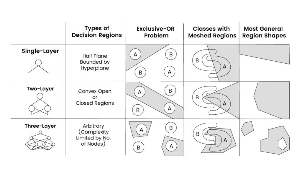
The XOR problem led to the development of multi-layer perceptrons (MLPs) and more advanced neural networks. By using multiple perceptrons and stacking them in layers, these networks can learn non-linear decision boundaries and solve more complex tasks.