5 - CNN for Localization and Weakly Supervised Localization

Data Preprocessing and Batch Normalization

Data preprocessing is an essential step in preparing data for gradient-based optimization techniques, particularly in deep learning models. Its primary purpose is to enhance the convergence of training algorithms and make the optimization process less sensitive to variations in the model’s parameters. This is achieved through normalization, which adjusts the data to have specific statistical properties, such as being zero-centered or scaled to a standard range. This adjustment improves the stability and efficiency of gradient descent.

Normalization

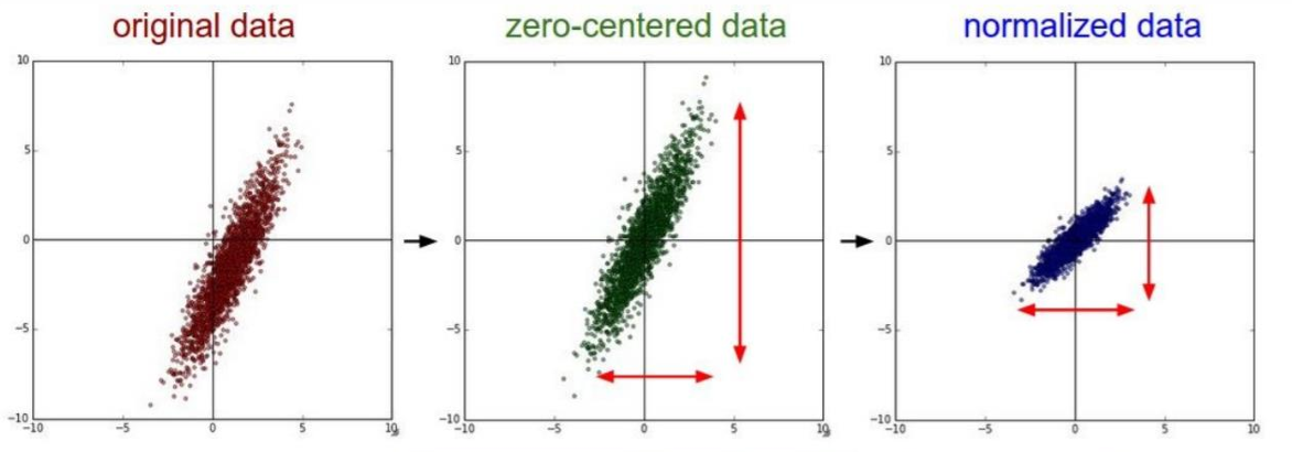
Normalization serves to align the data “around the origin,” typically by zero-centering or scaling its variance. Two widely-used methods are:

1. Zero-centering: This involves subtracting the mean of the data for each feature or pixel. Mathematically, it can be expressed as:

   where calculates the mean value of each feature or pixel.

2. Scaling by standard deviation: After zero-centering, the data can also be normalized by dividing by its standard deviation. This ensures that each feature or pixel has a standard deviation of 1:

PCA and Whitening

Principal Component Analysis (PCA) is often applied after zero-centering the data. It is a statistical procedure that transforms the data into a new coordinate system, where the axes (principal components) are orthogonal and aligned with the directions of maximum variance in the data. Two key outcomes of PCA in preprocessing include:

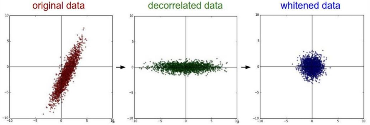
• Decorrelation: The covariance matrix of the data becomes diagonal, indicating that the transformed features are uncorrelated.
• Whitening: After decorrelation, whitening further scales the data so that its covariance matrix becomes the identity matrix. This step ensures that all features have unit variance.

However, in convolutional neural networks (CNNs), PCA and whitening are not commonly used. Instead, more straightforward normalization techniques, such as zero-centering and scaling, are typically preferred.

Normalization in Practice

The normalization strategy often depends on the specific architecture and dataset used. For instance, consider the preprocessing techniques used for the CIFAR-10 dataset (images of size ):

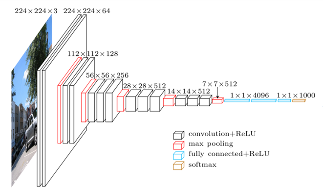
• AlexNet: Subtracts the mean image, a array computed across the entire training dataset.
• VGG: Subtracts the mean value computed independently for each channel (red, green, and blue), resulting in three scalar values.
• ResNet: Performs channel-wise normalization by subtracting the mean and dividing by the standard deviation for each channel. This requires six parameters: three mean values and three standard deviations.

These methods adjust the input data in a way that aligns with the design and training dynamics of each model.

Normalization introduces parameters into the machine learning pipeline, such as the mean and standard deviation of the training data. These parameters must be calculated exclusively from the training data and then applied consistently to the validation and test datasets. For example:

• Do not normalize before splitting the data: Computing normalization statistics on the entire dataset (before splitting into training, validation, and test sets) can lead to data leakage and overestimated performance metrics.
• Pretrained models: When using a pretrained model, it is crucial to apply the preprocessing function provided by the model’s developers. These functions ensure compatibility with the statistical properties of the data the model was originally trained on.

Batch Normalization

Batch Normalization is a widely used technique in deep learning to stabilize and accelerate training. It works by normalizing the activations of intermediate layers, ensuring that they have zero mean and unit variance during training. This normalization is performed over each mini-batch independently, making training less sensitive to initialization and enabling faster convergence.

Formula

Given a batch of activations , Batch Normalization applies the following transformation to normalize them:

Here:

• and are the mean and variance of the activations , computed for each mini-batch.
• is a small positive constant added to avoid division by zero.

This normalization is performed separately for each feature channel, ensuring that all channels contribute equally to the learning process.

After normalization, BN introduces a learnable parametric transformation:

where: and are learnable scale and shift parameters, respectively. These parameters allow the network to recover the original distribution of activations if necessary, ensuring flexibility.

During training, and are computed for each mini-batch. However, during testing, where batch sizes may differ or single samples are evaluated, BN uses running averages of and accumulated during training. This ensures consistent performance between training and inference.

Algorithm

The BN process for a mini-batch can be summarized as:

1. Compute the mini-batch mean:
2. Compute the mini-batch variance:
3. Normalize the activations:
4. Apply scaling and shifting:

In the testing phase, BN becomes a linear operator. The computation of normalization parameters is skipped, and the transformation relies entirely on the stored running averages of mean and variance. This makes the layer computationally efficient at inference time, as the operations can be fused with preceding fully-connected or convolutional layers.

Batch Normalization is most commonly applied between layers of a neural network to stabilize learning. While it is traditionally used between the fully connected (FC) layers of deep CNNs, it is also increasingly applied between convolutional layers. Its versatility and impact make it a core component of modern deep learning architectures.

Advantages	Limitations
Easier training for deep networks: BN reduces the sensitivity to initial weights and stabilizes learning.	Behavioral differences between training and testing: BN relies on mini-batch statistics during training but uses running averages during testing, which can lead to subtle bugs if not handled carefully.
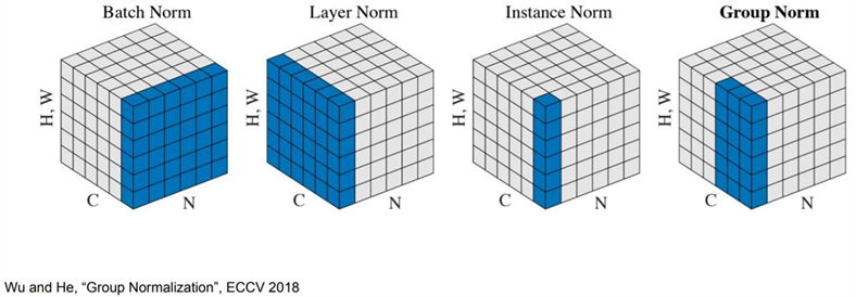
Improved gradient flow: It addresses the issue of vanishing and exploding gradients, especially in very deep networks.	Dependence on batch size: Small batch sizes can result in noisy statistics, reducing the effectiveness of BN. Alternative normalization techniques, such as Layer Normalization or Group Normalization, are better suited in such cases.
Faster convergence: The ability to use higher learning rates accelerates training.
Robustness: Networks become more resilient to poor initialization and hyperparameter selection.
Regularization: BN introduces slight noise in mini-batch statistics during training, acting as a form of regularization and reducing the need for dropout.
Efficiency at test time: The layer incurs no additional overhead during inference as its operations can be fused with the preceding layer.

CNN Visualization

Visualizing the inner workings of convolutional neural networks (CNNs) is essential for understanding how these models learn to extract features at different layers. From low-level patterns in the early layers to high-level representations in the deeper ones, visualization techniques provide insights into the network’s decision-making process.

Visualization of Filters and Features

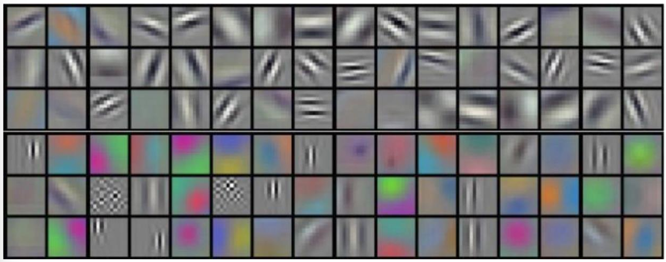
In early layers like the first convolutional layer of AlexNet, the filters are visualized as kernels (RGB images). These filters act as templates that match simple, low-level features such as edges, corners, and textures. This is because the convolution operation is closely related to template matching, where filters detect patterns in the input image by producing high responses to regions that closely match their structure.

However, as we move deeper into the network, the features become increasingly abstract and difficult to interpret. Deep layers detect complex patterns, such as parts of objects or high-level semantic features, which are less intuitive to visualize.

One way to interpret deeper layers is by identifying “maximally activating patches.” This technique involves finding input regions that activate specific neurons most strongly, providing a window into what a neuron “sees.” The process is as follows:

1. Neuron Selection: Choose a neuron in a deep layer of a pre-trained CNN (e.g., trained on ImageNet).
2. Activation Extraction: Pass a set of input images through the network and store the activations for the selected neuron.
3. Maximally Activating Image: Identify the image that produces the maximum activation for the chosen neuron.
4. Receptive Field Identification: Highlight the region (patch) of the input image corresponding to the receptive field of the selected neuron.
5. Iterative Analysis: Repeat this process for multiple neurons to understand their respective roles.

Each row in the resulting visualization corresponds to outputs from different filters of the same layer, revealing the diversity of patterns the filters are tuned to detect.

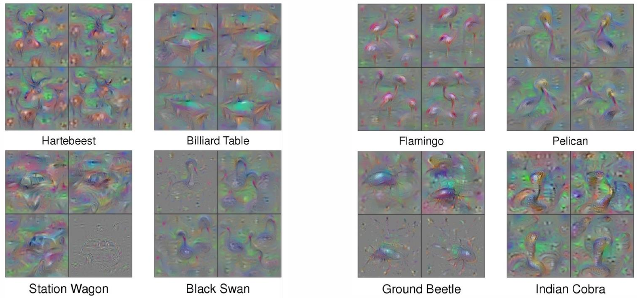
Another approach to understanding what a neuron “prefers” is to compute an input image that maximally activates it. This technique uses gradient ascent and is particularly effective for visualizing features of deep layers:

1. Compute Gradients: Select a neuron and calculate the gradient of its activation value with respect to the input image. This is feasible because all operations in a CNN are differentiable.
2. Gradient Ascent: Modify the input image slightly in the direction of the gradient to increase the activation of the neuron. This is the inverse of gradient descent, as we aim to maximize (not minimize) the function.
3. Iterate: Repeatedly adjust the input using gradient ascent to find the image that most strongly activates the neuron.
4. Regularization: To ensure the generated image looks natural and interpretable, add a regularization term to penalize unnatural patterns: where is the score for a class , is a regularization parameter, and encourages smoothness in the image.

Layer-Specific Responses

• Shallow Layers: Respond to low-level features like edges, textures, and simple color patterns.
• Intermediate Layers: Capture mid-level features such as shapes, contours, or combinations of basic patterns.
• Deep Layers: Encode high-level semantic concepts such as object parts or categories.

To understand how a network predicts a specific class, we can apply gradient ascent before the softmax layer to maximize the score for a target class . This process generates an input image that strongly activates the network’s prediction for that class. By iterating this process for various classes, we obtain a set of visualizations that represent what the network “thinks” each class looks like.

Localization in Object Detection

Localization in computer vision involves identifying the position of a specific object within an image and assigning it to a predefined category. Unlike simple classification tasks where the entire image is assigned a label, localization combines classification with spatial understanding, requiring the model to predict a bounding box around the object of interest.

The localization task is generally divided into two objectives:

1. Object Classification: The model must assign the input image to a specific class within a fixed set of categories, such as “cat,” “car,” or “person.”
2. Bounding Box Prediction: Simultaneously, the model predicts the coordinates of a bounding box enclosing the object. These coordinates typically include:
   • : The center of the bounding box.
   • : The height of the bounding box.
   • : The width of the bounding box.

To train a model for localization, the dataset must consist of annotated images. Each annotation should include:

1. A class label identifying the category of the object in the image.
2. A bounding box specifying the object’s position and size in terms of .

For more advanced problems, such as human pose estimation, the annotations may involve regression over more complex geometries, such as keypoints for body parts or skeletal structures.

Bounding Box Estimation

Bounding box estimation is framed as a regression problem. The model is trained to predict the bounding box coordinates for the object in an image , where and represent the height and width of the image. The task can be expressed as a mapping function:

This is typically achieved using a neural network with an output layer that predicts four continuous values (the bounding box coordinates). A practical implementation in TensorFlow/Keras might look as follows:

# Define the output layer: 4 real numbers for bounding box coordinates with linear activation
output = tf.keras.layers.Dense(4, activation='linear', name='regressor')(x)
 
# Connect input and output through the Model class
regressor_model = tf.keras.Model(inputs=inputs, outputs=output, name='regressor_model')
 
# Compile the model using Mean Squared Error (MSE) as the loss function
regressor_model.compile(loss=tf.keras.losses.MeanSquaredError(), optimizer=tf.keras.optimizers.Adam())

Here, the network’s loss function (Mean Squared Error) measures the deviation between the predicted and ground truth bounding box coordinates.

Combined Classification and Localization

In many practical scenarios, the task requires not just bounding box prediction but also simultaneous classification of the object within it. The output for such a model includes both:

1. Bounding box coordinates: .
2. Object label , from a set of categories .

This setup creates a multi-task learning problem, as the outputs—bounding box coordinates (regression) and class labels (classification)—are of different natures. The combined task can be expressed as:

To handle this, the network typically includes separate heads for each task:

• A regression head for predicting bounding box coordinates.
• A classification head with a softmax activation to predict the category label.

The total loss function is a weighted combination of the two losses:

where and are weights balancing the importance of the two tasks.

Multitask Learning

Multitask learning allows a single neural network to predict multiple outputs simultaneously, such as class labels and bounding box coordinates. This approach is computationally efficient and enables the network to learn shared features for both tasks, leading to better generalization.

The network is designed with two distinct “heads”:

1. Classification Head: Predicts the object class using a softmax activation. The corresponding loss is the categorical cross-entropy, denoted as .
2. Regression Head: Predicts the bounding box coordinates using a regression loss, typically (Mean Squared Error) or norm. The regression loss is denoted as and defined as:

The overall multitask loss is a weighted combination of the two losses:

where is a hyperparameter balancing the importance of classification and localization. Fine-tuning is crucial, as improper weighting may lead to suboptimal performance. Cross-validation is recommended to determine the best value, though evaluating directly for different values might not always yield meaningful insights.

In practice, multitask models use a shared backbone network to extract features, followed by two specialized heads for classification and localization. For example, consider using MobileNet as a backbone:

# Define inputs and add MobileNet as feature extractor
inputs = tf.keras.Input(shape=train_images.shape[1:])
x = mobile(inputs)
 
# Add classification head for multiclass classification
class_outputs = tf.keras.layers.Dense(2, activation='softmax', name='classifier')(x)
 
# Add regression head for bounding box prediction
box_outputs = tf.keras.layers.Dense(4, activation='linear', name='localizer')(x)
 
# Create and compile the multitask model
object_localization_model = tf.keras.Model(inputs=inputs, outputs=[class_outputs, box_outputs], name='object_localization_model')
object_localization_model.compile(loss=[tf.keras.losses.CategoricalCrossentropy(), 
										tf.keras.losses.MeanSquaredError()],
								  optimizer=tf.keras.optimizers.Adam()
)

A simpler, “quick and dirty” implementation for multitask learning assumes binary classification and normalized bounding box coordinates (values in relative to the image size). The bounding box prediction is constrained within the image boundaries using sigmoid activations.

# Define the model architecture
inputs = tf.keras.Input(shape=(img_size, img_size, 3))
x = mobile(inputs)
x = tf.keras.layers.Dropout(0.5)(x)
 
# Binary classification head
class_output = tf.keras.layers.Dense(1, activation='sigmoid', name='classifier')(x)
 
# Bounding box regression head
box_output = tf.keras.layers.Dense(4, activation='sigmoid', name='localizer')(x)
 
# Combine inputs and outputs into a multitask model
object_localization_model = tf.keras.Model(inputs=inputs, 
										   outputs=[class_output, box_output], 
										   name='object_localization_model')
object_localization_model.compile(loss=tf.keras.losses.BinaryCrossentropy(), 
								  optimizer=tf.keras.optimizers.Adam())
object_localization_model.summary()

While this approach is straightforward, it has limitations:

1. It cannot handle multiclass classification.
2. Bounding box predictions are constrained within the image and cannot handle out-of-bound cases.

To implement a fully flexible multitask loss, you may need to modify the training loop manually.

Human Pose Estimation

Human pose estimation is a specific type of localization task where the goal is to predict the positions of key body joints. This task is typically formulated as a regression problem in which a convolutional neural network (CNN) predicts a vector of coordinates, representing the joint positions (e.g., wrists, elbows, knees) in the image.

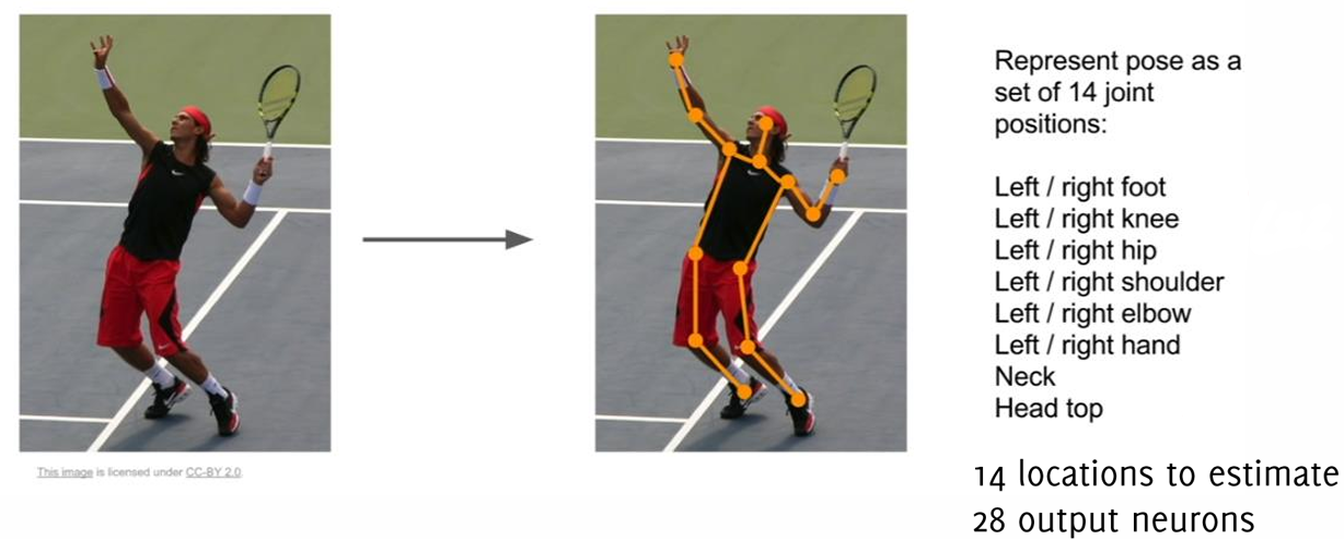
Key Steps in Pose Estimation:

1. Input: The entire image is fed into the network to provide full spatial context for predicting joint positions.
2. Output: The network predicts normalized joint locations relative to the bounding box enclosing the person.
3. Loss Function: Training uses an regression loss: where represents ground truth joint coordinates and represents predicted values.

Training Strategies:

• Data Augmentation: Techniques like translation and flipping are used to reduce overfitting and improve robustness.
• Transfer Learning: Pretrained classification networks (e.g., AlexNet) are fine-tuned for pose estimation to leverage existing feature representations.
• Iterative Refinement: Networks can be trained sequentially, refining joint predictions using localized crops of the input image.

Saliency Maps and Weakly-Supervised Localization

In supervised learning, a model that performs inference from an input space to an output space , represented as , requires a training set . This training set consists of paired input-output data of the same type as the target inference task. However, for certain tasks such as image segmentation, the process of obtaining these annotations can be prohibitively expensive and time-consuming due to the detailed labeling required.

Weak supervision offers an alternative approach by enabling a model to perform inference on tasks in the output domain using labels that are easier to acquire in a related but distinct domain . In this case, while the inference task remains , the training set instead consists of pairs from , where . This paradigm reduces the annotation burden by leveraging less precise but more readily available labels.

One specific application of weak supervision is weakly-supervised localization. Here, the goal is to train a model capable of performing localization (predicting bounding boxes) without requiring images annotated with bounding boxes during training. Instead, the training data is annotated for classification, with image-label pairs , where is the class label, but no localization information is provided. Remarkably, this approach enables the training of a classifier that simultaneously provides estimates of object locations, demonstrating the dual functionality of classification and localization.

The Global Average Pooling (GAP) Layer

A key architectural component enabling weakly-supervised localization is the Global Average Pooling (GAP) layer. Consider a convolutional neural network (CNN) architecture that ends with a block of feature maps, denoted as , where each feature map has a resolution that is approximately similar to the input image. After these feature maps, a GAP layer computes the spatial average of each feature map, producing scalar values:

These aggregated values summarize the global contributions of each feature map. Subsequently, a fully connected (FC) layer is added and trained. This FC layer computes scores for each class as a weighted sum of the GAP outputs:

where are trainable parameters representing the importance of the ^th feature map for class . The scores are then transformed into class probabilities via the softmax function:

The weights effectively encode how each feature map contributes to the prediction of class .

Importantly, the GAP layer's structural simplicity acts as a regularizer, reducing the risk of overfitting while maintaining the CNN's capacity to localize discriminative regions in the input image.

The computation of can be reformulated to reveal the spatial contributions of individual activations:

This perspective highlights that aggregates contributions from all spatial locations , weighted by . From this formulation, the Class Activation Map (CAM) for class is derived:

The CAM directly indicates the importance of the activation at spatial location for predicting class . This visualization capability allows CNNs to highlight the image regions most critical for a given prediction.

Beyond its role in structural regularization, the GAP layer equips CNNs with a remarkable ability to retain localization information through the final layers. With minimal architectural modifications, CNNs trained for object categorization can also localize the discriminative regions responsible for their predictions. This capability extends to diverse applications, such as action classification, where the network identifies objects interacting with humans rather than focusing solely on the human figure.

Class Activation Mapping (CAM)

Class Activation Mapping (CAM) is a technique used to identify which regions of an image a neural network focuses on when making predictions. It highlights the discriminative areas that contribute the most to the classification decision. CAM is computationally straightforward and requires the following components:

1. A classifier that includes a Global Average Pooling (GAP) layer.
2. A fully connected (FC) layer positioned after the GAP layer.
3. A minor modification to extract saliency maps from the model.

The final layer weights encode the relevance of each feature map for the final prediction. To match the resolution of the input image, the resulting CAM (which is typically smaller than the input image) is usually upsampled using methods like bilinear interpolation.

Steps for Computing CAM:

1. Classifier Design: CAM can be implemented in any pre-trained network as long as all fully connected layers at the end are replaced. The new FC layer used for CAM is minimal, with only a few neurons and no hidden layers. However, this simplification might reduce classification performance; for instance, removing the dense layers from VGG nets results in a significant parameter loss, approximately 90%.

2. Heatmap Visualization: CAM outputs are low-resolution maps that are upsampled to match the original image size. Thresholding can be applied (e.g., values of ) to isolate the most relevant regions. The largest connected component of the thresholded map often aligns with the object of interest.

3. Pooling Variants: GAP encourages the model to consider all regions of the object, as all activations contribute to the final classification. In contrast, Global Max Pooling (GMP) highlights only the most discriminative features, focusing on highly specific areas.

The resolution of CAMs can be enhanced by positioning the GAP layer earlier in the network, at layers with larger spatial dimensions. However, this comes at the cost of reduced semantic information in the feature maps, as higher-resolution layers typically capture more granular details rather than high-level semantics.

For instance, networks trained with GAP layers are effective at localizing objects in images even when trained for classification tasks. This is because GAP forces the network to focus on the entirety of an object rather than specific parts, making CAM suitable for weakly supervised tasks such as object localization.

The following Python function demonstrates how to compute CAM for an input image using a pre-trained network, such as MobileNetV2:

def compute_CAM(model, img): 
    # Expand image dimensions to fit the model input shape 
    img = np.expand_dims(img, axis=0) 
    
    # Predict to get the winning class 
    predictions = model.predict(img, verbose=0) 
    label_index = np.argmax(predictions) 
    
    # Get the weights of the fully connected layer (before softmax) 
    class_weights = model.layers[-1].get_weights()[0] 
    
    # Extract the weights corresponding to the winning class 
    class_weights_winner = class_weights[:, label_index] 
    
    # Retrieve the final convolutional layer 
    final_conv_layer = tfk.Model(
        inputs=model.get_layer('mobilenetv2_1.00_224').input,
        outputs=model.get_layer('mobilenetv2_1.00_224').get_layer('Conv_1').output
    )
    
    # Compute the convolutional outputs 
    conv_outputs = final_conv_layer(img) 
    conv_outputs = np.squeeze(conv_outputs) 
    
    # Upsample the outputs to match the input image resolution 
    mat_for_mult = scipy.ndimage.zoom(conv_outputs, (32, 32, 1), order=1) 
    mat_for_mult = mat_for_mult.reshape((256*256, 1280)) 
    
    # Compute the CAM by applying the class weights 
    final_output = np.dot(mat_for_mult, class_weights_winner) 
    
    # Reshape the CAM to the input image dimensions 
    final_output = final_output.reshape(256, 256) 
    
    return final_output, label_index, predictions

1. Weight Extraction: The weights from the fully connected layer, corresponding to the predicted class, are retrieved. These weights determine how each feature map contributes to the class prediction.
2. Convolutional Outputs: The output of the final convolutional layer is extracted and upsampled to match the spatial dimensions of the input image.
3. Weighted Sum: The CAM is calculated as the weighted sum of the upsampled feature maps, where the weights are the class-specific weights from the FC layer.
4. Heatmap Generation: The resulting CAM is reshaped and can be visualized as a heatmap overlaid on the original image, providing insights into the regions influencing the prediction.

Explaining Neural Network Predictions

Deep neural networks (DNNs) are powerful computational models that can learn complex patterns from data. However, they contain millions of parameters, making their internal operations opaque and difficult to interpret. This lack of transparency raises concerns about their reliability, especially in critical applications such as the medical domain (e.g., diagnostics) or financial services (e.g., blocking credit cards). In these high-stakes scenarios, blind trust in neural network decisions is dangerous, leading to a growing demand for methods that explain their predictions.

Researchers are actively developing techniques to demystify neural network decision-making, aiming to provide interpretable explanations that build trust and enable debugging. Among these methods, Grad-CAM and CAM-based approaches stand out as robust tools for visualizing how neural networks make decisions.

Grad-CAM and CAM-Based Techniques

Grad-CAM (Gradient-weighted Class Activation Mapping) extends the principles of CAM by introducing flexibility and broader applicability. Unlike CAM, Grad-CAM does not require architectural modifications, allowing it to work with a wide range of pre-trained networks. The essence of Grad-CAM lies in generating class-specific heatmaps that highlight the most relevant regions in the input image for a given prediction.

The computation of Grad-CAM involves two main steps:

1. Gradient Weight Calculation: Grad-CAM computes the importance of each feature map by averaging the gradients of the class score with respect to activations:

   Here, represents the spatial dimensions of the feature map.

2. Heatmap Generation: The importance weights are combined with their respective feature maps, followed by the application of a ReLU function to produce the final class-specific heatmap:

The resulting heatmap is class-discriminative and reveals which parts of the input image are most influential in the network’s prediction.

Grad-CAM heatmaps have two important characteristics:

• Class Discrimination: They highlight regions corresponding to the predicted class, making it easier to understand the network’s decision.
• Fine-Grained Detail: High-resolution heatmaps are crucial for applications such as medical imaging, where precision is essential to identify subtle abnormalities.

Augmented Grad-CAM: Enhancing Heatmap Resolution

One limitation of Grad-CAM is that the resolution of the heatmaps is tied to the spatial dimensions of the final convolutional layer, which are typically lower than the input image’s resolution. Augmented Grad-CAM addresses this by using data augmentation to enhance the resolution of the generated heatmaps.

The key idea of Augmented Grad-CAM is to increase heatmap resolution by leveraging multiple augmented versions of the same input image. The process begins by applying an augmentation operator , which introduces random transformations (e.g., rotations and translations) to the input image . Each augmented version of the input is then processed through the network, producing a low-resolution saliency map via Grad-CAM.

These low-resolution maps are treated as the results of a common downsampling operator , applied to various perturbed versions of a high-resolution saliency map . By combining the saliency maps from different augmented inputs, Augmented Grad-CAM reconstructs a more detailed and accurate high-resolution heatmap.

Advantages of Augmented Grad-CAM:

• Improved Resolution: The reconstructed high-resolution heatmap captures finer details, making it particularly valuable for applications requiring high precision, such as industrial quality control or medical imaging.
• Robust Explanations: The use of multiple augmented inputs ensures that the generated heatmaps are less sensitive to noise or individual perturbations, providing a more stable and reliable interpretation of the network’s behavior.

Grad-CAM heatmaps are inherently low-resolution due to the spatial dimensions of the final convolutional layer. To enhance these heatmaps, we model them as the result of a linear downsampling operator , which maps an unknown high-resolution heatmap to a lower-resolution heatmap . The task of super-resolution for heatmaps is then formulated as solving the following inverse problem:

where:

• is an augmentation operator that applies random transformations (e.g., rotations, translations) to the high-resolution heatmap ,
• is an anisotropic total variation regularization term that preserves the edges in the high-resolution heatmap,
• and are hyperparameters controlling the regularization strength.

The total variation regularization term is defined as:

where and are the gradients of along the and axes. This term ensures that the reconstructed heatmap maintains sharp edges, which are critical for accurate localization.

The optimization problem is solved using Subgradient Descent, as the objective function is convex but non-smooth. This approach ensures computational efficiency and convergence to a global minimum.

Advanced Gradient-Based Saliency Maps: Grad-CAM++ and Smooth Grad-CAM++

Building on Grad-CAM, advanced techniques improve localization accuracy and interpretability by refining how heatmaps are generated.

Grad-CAM++ extends Grad-CAM by incorporating higher-order derivatives of the class score with respect to feature maps . This approach increases the localization accuracy, especially in cases where multiple occurrences of the same object are present in the image. The weights in Grad-CAM++ are computed as:

This formulation ensures a more precise focus on discriminative regions while maintaining computational feasibility.

Smooth Grad-CAM++ further enhances Grad-CAM++ by averaging multiple heatmaps generated from noisy versions of the same input image. This averaging reduces noise and improves robustness, leading to more reliable explanations.

An alternative to gradient-based methods, perturbation-based saliency maps identify influential image regions by systematically modifying the input and observing changes in the class score. A notable example is RISE (Randomized Input Sampling for Explanations), which applies random perturbations (e.g., masking parts of the image) to pinpoint areas critical for the network’s decision. This approach is particularly useful for explaining predictions in a class-specific manner.

Perception Visualization (PV)

Perception Visualization (PV) offers a complementary approach to saliency maps by inverting latent representations within the neural network. Instead of directly highlighting input regions, PV reconstructs input-like visualizations that explain the network’s internal features. This method provides deeper insights into how the network processes data.

Studies have demonstrated that PV significantly enhances human interpretability of neural network predictions. For instance, in a study involving approximately 100 subjects, PV helped users better understand cases where the model had made an error. By visualizing the network’s latent reasoning, PV enables a more intuitive grasp of decision boundaries and potential flaws in the model’s logic.