Autoencoders are a class of neural networks designed primarily for data reconstruction and are commonly used in unsupervised learning tasks. The fundamental purpose of an autoencoder is to learn an efficient encoding of input data and subsequently use that encoding to reconstruct the input as accurately as possible. This property allows autoencoders to identify patterns and structures within data, often serving as a foundation for tasks such as dimensionality reduction, anomaly detection, and generative modeling.
Structure and Functionality of Autoencoders
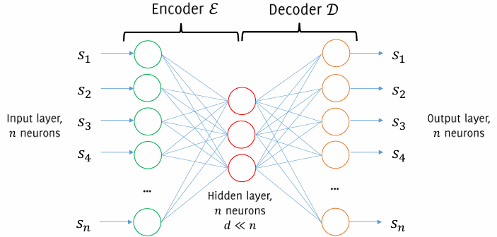
An autoencoder typically consists of two primary components: an encoder and a decoder. The encoder, denoted as
The training process involves optimizing the parameters of both the encoder and decoder to minimize a reconstruction loss function. For a batch of data points
This optimization is performed using standard backpropagation techniques, such as stochastic gradient descent (SGD), and aims to approximate an identity mapping through the encoder-decoder pipeline. Notably, no external labels are required during training; the autoencoder’s objective is purely to reconstruct its inputs.
Insights into Latent Representations
The latent representation
plays a critical role in the effectiveness of an autoencoder. Since the dimensionality of the latent space is typically much smaller than that of the input space , the autoencoder is compelled to learn a compact and meaningful representation of the input. This constraint often forces the network to capture the most salient features of the data, discarding redundant or noisy information. However, autoencoders do not always achieve perfect reconstruction due to this dimensionality reduction. Instead, the network’s design encourages the latent space to encode meaningful variations in the data. For instance, in image data, the latent representation might capture key features like edges, textures, or object outlines, while ignoring finer details.
Regularization in Autoencoders
To further refine the latent representation or enhance the quality of reconstruction, regularization techniques can be introduced. A common approach is to add a penalty term to the loss function, represented as
- Latent Space Properties: Encouraging sparsity in the latent representation or enforcing it to follow a specific distribution, such as a Gaussian, can make the encoding more interpretable or suitable for downstream tasks.
- Reconstruction Characteristics: Applying regularization to the reconstructed output can enhance its quality by enforcing smoothness or emphasizing certain features, such as sharp edges in image data.
The representational power of an autoencoder can be significantly enhanced by introducing depth in its architecture. Deep autoencoders, which consist of multiple hidden layers within both the encoder and decoder, allow for the learning of highly nonlinear mappings. Such architectures are capable of capturing intricate data structures and are particularly effective for complex datasets.
Additionally, for data with spatial hierarchies, such as images, convolutional layers can be used in place of fully connected layers. This results in convolutional autoencoders, where convolutional layers in the encoder extract local patterns, and transposed convolutions in the decoder reconstruct the input. These architectures are particularly adept at preserving spatial relationships and are widely applied in image denoising, super-resolution, and similar tasks.
Training Autoencoders
An autoencoder consists of two main components: the encoder, which compresses input data into a lower-dimensional latent representation, and the decoder, which reconstructs the input data from the latent space. The encoder compresses high-dimensional input data into a compact latent representation.
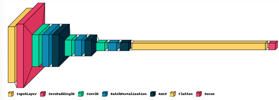
In the implementation:
input_layer = tfkl.Input(shape=enc_input_shape, name='input_layer')

# block of conv+batchnorm+relu
x = tfkl.Conv2D(64, 3, padding='same', strides=2)(input_layer)
x = tfkl.BatchNormalization()(x)
x = tfkl.ReLU()(x)

# Another block of conv+batchnorm+relu
# Another block of conv+batchnorm+relu

# flattening and a dense layer to the latent_dim
x = tfkl.Flatten()(x)
output_layer = tfkl.Dense(enc_output_shape, name='output_layer')(x)

# the value returned by the output layer is the latent representation
# Connect input and output through the Model class
model = tfk.Model(inputs=input_layer, outputs=output_layer, name='encoder')-
Input Layer: The encoder begins with an input layer that accepts data in a predefined shape (
enc_input_shape). -
Convolutional Block:
- A 2D convolution layer extracts spatial features while reducing spatial resolution due to the stride value.
- Batch Normalization normalizes activations to stabilize and accelerate training.
- ReLU Activation introduces nonlinearity to enable the model to learn complex patterns.
-
Further Feature Extraction: Additional convolutional blocks can be added in the same format (Conv2D + BatchNormalization + ReLU) to deepen the encoder and enhance feature extraction.
-
Latent Representation:
- The output is flattened into a vector using the
Flattenlayer. - A final dense layer maps the flattened features to the desired latent space dimension (
enc_output_shape). This dense layer’s output forms the latent representation.
- The output is flattened into a vector using the
The encoder’s architecture is encapsulated in a Keras Model, which maps the input layer to the output latent representation.
The decoder reconstructs the input data from the latent representation.

It reverses the transformations performed by the encoder:
input_layer = tfkl.Input(shape=dec_input_shape, name='input_layer')

# add a dense layer from the latent representation to a larger vector
x = tfkl.Dense(n_rows*n_cols*n_channels)(input_layer)
x = tfkl.BatchNormalization()(x)
x = tfkl.ReLU()(x)

# invert the flattening by reshaping
x = tfkl.Reshape((n_rows, n_cols, n_channels))(x)

# upsampling block: upsampling + convolution + batchnorm + relu
x = tfkl.UpSampling2D()(x)
x = tfkl.Conv2D(128, 3, padding='same')(x)
x = tfkl.BatchNormalization()(x)
x = tfkl.ReLU()(x)

# Another upsampling block: upsampling + convolution + batchnorm + relu
# Another upsampling block: upsampling + convolution + batchnorm + relu

# the last block is a convolution returning to the image domain
x = tfkl.Conv2D(dec_output_shape[-1], 3, padding='same')(x)
x = tfkl.Activation('sigmoid')(x) #’ by doing so we clip values, linear is also fine

# Connect input and output through the Model class
model = tfk.Model(inputs=input_layer, outputs=output_layer, name='decoder')-
Input Layer: The decoder takes the latent representation (
dec_input_shape) as input. -
Upscaling the Latent Representation:
- A Dense Layer expands the latent vector back into a larger dimensional vector matching the flattened size of the original input.
- Batch normalization and ReLU activation are applied here for stability and nonlinearity.
-
Reshaping: The expanded vector is reshaped to match the original spatial dimensions using the
Reshapelayer. -
Upsampling Blocks: Each block consists of UpSampling2D, Conv2D, BatchNormalization, and ReLU layers, progressively increasing the spatial resolution while refining the reconstructed features.
-
Final Reconstruction:
- A final convolution layer maps the decoder’s output back to the input domain.
- A Sigmoid activation ensures the output values are clipped between 0 and 1, suitable for normalized image data.
As with the encoder, the decoder’s architecture is encapsulated in a Keras Model.
Autoencoder
def get_autoencoder(ae_input_shape=input_shape, ae_output_shape=input_shape):
	tf.random.set_seed(seed)

	# invoke functions to instantiate models
	encoder = get_encoder()
	decoder = get_decoder()

	# assemble the network
	input_layer = tfkl.Input(shape=ae_input_shape)
	z = encoder(input_layer)
	output_layer = decoder(z)

	model = tfk.Model(inputs=input_layer, outputs=output_layer, name='autoencoder')

	return model

# instantiate the autoencoder
autoencoder = get_autoencoder()
autoencoder.summary()
tfk.utils.plot_model(autoencoder, show_shapes=True, expand_nested=True, to_file='autoencoder.png')
The autoencoder combines the encoder and decoder into a single end-to-end model:
- Input Layer: Accepts the input data (
ae_input_shape). - Encoder Integration: The input passes through the encoder, producing the latent representation.
- Decoder Integration: The latent representation is passed to the decoder, which reconstructs the input.
- Model Definition: A Keras
Modelcombines these components, linking the input to the reconstructed output.
The assembled model is instantiated using the get_autoencoder function.
Training the Autoencoder
The training process involves minimizing the reconstruction loss between the input and its reconstruction. The steps include:
# define training options
learning_rate = 1e-3
optimizer = tf.optimizers.Adam(learning_rate)

# the autoencoder needs to be trained by minimizing a reconstruction loss
autoencoder.compile(optimizer=optimizer, loss=tfk.losses.MeanSquaredError(), metrics=['mse', 'mae'])

# train the autoencoder
autoencoder.fit(
	X_train, # the input
	X_train, # the target for the autoencoder is the input itself
	batch_size=batch_size,
	epochs=epochs,
	validation_data=(X_val,X_val), # the target for the autoencoder is the input itself
	callbacks=[tfk.callbacks.EarlyStopping(monitor='val_loss', patience=10, restore_best_weights=True),
		tfk.callbacks.ReduceLROnPlateau(monitor='val_loss', patience=5, factor=0.5, min_lr=1e-5),
	]
)-
Compile the Model:
- An Adam optimizer with a learning rate of
is used for efficient gradient updates. - The Mean Squared Error (MSE) loss measures the difference between the input and reconstructed output.
- Additional metrics like MSE and Mean Absolute Error (MAE) track training performance.
- An Adam optimizer with a learning rate of
-
Training:
- The model is trained using the
fitmethod, where both inputs and targets are the same (unsupervised learning). - Early stopping monitors the validation loss, halting training if it doesn’t improve for 10 epochs.
- A learning rate reduction callback decreases the learning rate by half if validation loss stagnates for 5 epochs, preventing overfitting.
- The model is trained using the
-
Validation: A separate validation set evaluates the model during training to ensure generalizability.
Latent Representation
The size of the latent representation in an autoencoder directly influences the quality of the reconstructions. A larger latent space provides more capacity to encode information, resulting in more accurate reconstructions. For instance:
- When the latent space dimension
, the encoded representation is highly compressed, limiting the autoencoder’s ability to capture complex details, and thus the reconstructed images may lose fidelity. 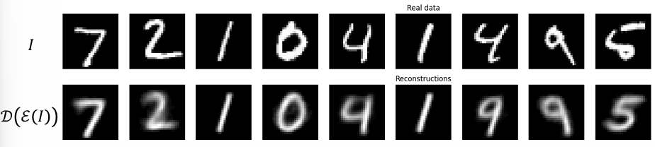
- When
, the larger latent space allows the model to encode finer details, producing higher-quality reconstructions. 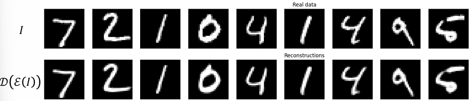
In the limiting case, where the latent dimension matches the input dimension, the autoencoder effectively learns the identity mapping, perfectly reconstructing the input. However, this defeats the purpose of learning meaningful or compact representations.
This relationship between latent space size and reconstruction quality highlights the trade-off between compression and reconstruction fidelity. Smaller latent dimensions emphasize feature extraction, while larger ones prioritize reconstruction accuracy.
Autoencoders for Classifier Initialization
Autoencoders are particularly valuable in scenarios where labeled data is scarce. When dealing with a large unlabeled dataset
- Unsupervised Pretraining: Train the autoencoder on the unlabeled dataset
to learn meaningful latent representations. - Encoder Retention: After training, discard the decoder and retain the encoder weights
, which now contain a compact representation of the input data. - Classifier Integration: Add a fully connected (FC) layer to the encoder’s output for classification. This FC layer maps the latent representation to class labels.
- Fine-tuning: Using the small labeled set
, fine-tune the autoencoder, optimizing both the encoder weights and the newly added classifier. If is sufficiently large, the encoder can undergo additional training for better alignment with the labeled data.
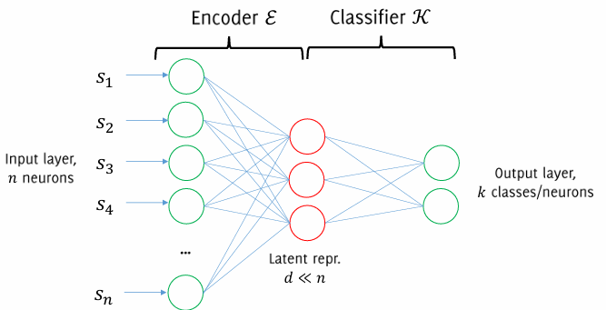
This process leverages transfer learning, as the encoder, pretrained on
- Improved Initialization: The pretrained encoder provides a meaningful starting point, reducing training time and improving convergence.
- Overfitting Mitigation: The latent representations are less prone to overfitting, as they are learned from a broader dataset, capturing general patterns.
Sampling the Latent Space
Using autoencoders as generative models involves sampling the latent space to produce new data. A naive approach is:
- Train the Autoencoder: Learn latent representations using the unlabeled dataset
. - Discard the Encoder: Use only the trained decoder for data generation.
- Random Sampling: Generate random vectors
, which are fed into the decoder to produce new outputs.
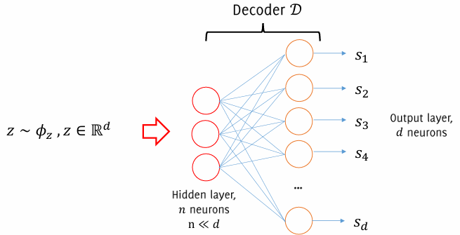
However, this approach faces challenges because the latent space is not uniformly populated:
- Unknown Distribution: The actual distribution of valid latent representations is typically unknown and difficult to estimate accurately.
- High Dimensionality Issues: As the latent space dimension
increases, high-density regions become sparse, leading to samples from less populated areas. These regions often do not correspond to meaningful inputs, resulting in unrealistic outputs.
Example: Latent Space Sampling in MNIST
For a low-dimensional latent space (
), it is possible to define a grid covering the “populated” regions of the latent space. This allows the decoder to generate valid outputs that correspond to meaningful samples. However, as grows, the probability of sampling a valid region decreases significantly, making this approach less effective.
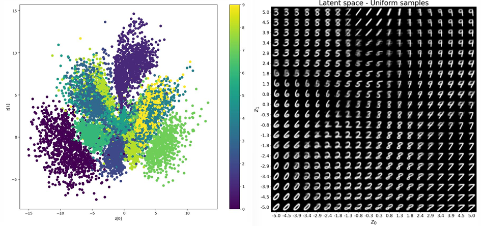
Variational Autoencoders (VAEs) and Latent Space Regularization
Variational Autoencoders address these issues by regularizing the latent space. They enforce the latent representations to follow a known distribution, typically a Gaussian. This involves:
- Adding a regularization term to the loss function that minimizes the divergence between the latent distribution and the target Gaussian distribution.
- Sampling latent representations
from the Gaussian distribution during generation.
This structured latent space ensures that random samples from the distribution correspond to realistic outputs. In addition to providing accurate reconstructions, VAEs are considered generative models, capable of producing new, meaningful data.