4.4 - Convolutional Neural Networks for Semantic Segmentation

Image segmentation is a fundamental task in computer vision aimed at dividing an image into meaningful segments or regions based on pixel similarities. The objective of image segmentation is to identify and group pixels that “go together,” making it easier to recognize and process objects within an image. By grouping similar-looking pixels, segmentation enhances the efficiency of image analysis, enabling systems to separate an image into distinct, coherent objects.

Conceptually, image segmentation can be viewed as a clustering problem, where the goal is to partition an image , defined over a domain , into regions such that:

This indicates that each pixel belongs to a unique segment, ensuring that no regions overlap. Image segmentation can be divided into two primary types: unsupervised and supervised (or semantic) segmentation. In this context, we focus on supervised segmentation.

Semantic Segmentation

Semantic segmentation is a form of supervised image segmentation where each pixel in the image is associated with a specific category or label. Given an image , the aim is to assign a label from a predefined set to each pixel , effectively creating a map where each pixel holds the estimated class it belongs to. In semantic segmentation, there is no differentiation between individual instances within a class; for instance, if multiple people appear in an image, they will all be labeled as “person” without distinguishing among them. This is in contrast to instance segmentation, which identifies separate instances of each object class.

For example, given a set of labels such as , semantic segmentation transforms an image into a labeled map , where denotes the label for the pixel at position . To achieve this, we rely on a training set , where represents ground truth annotations that have been manually labeled to serve as references during model training.

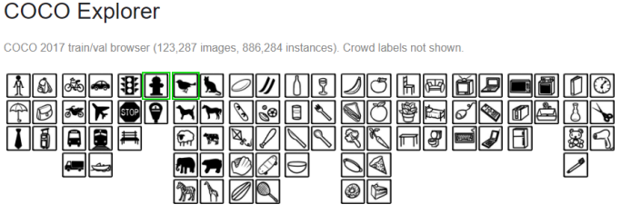
One of the most widely used datasets for semantic segmentation is the Microsoft COCO (Common Objects in Context) dataset. This large-scale dataset is designed for various object detection, segmentation, and image captioning tasks, offering rich contextual information and a high level of diversity. The COCO dataset comprises images, with over labeled images, and includes million object instances across 80 object categories and 91 background or “stuff” categories. Additionally, each image is accompanied by multiple captions and annotated human keypoints, making COCO a versatile resource for training deep learning models in semantic segmentation.

Semantic Segmentation with Fully Convolutional Networks (FCNs)

Fully Convolutional Networks (FCNs) have become a standard approach for semantic segmentation, aiming to classify every pixel in an image. Unlike traditional CNNs used for image classification, FCNs eliminate fully connected layers, focusing instead on convolutional layers to retain spatial information throughout the network. The design of FCNs involves a unique combination of downsampling and upsampling stages, balancing global feature extraction with precise, pixel-level predictions.

Balancing Depth and Spatial Resolution

In semantic segmentation, maintaining a balance between high-level semantic information and spatial accuracy is essential. Deep convolutional layers capture abstract, global context from an image, helping to identify what is present (e.g., whether an object is a person, car, or tree). However, the downsampling operations often result in a loss of fine spatial detail, making it challenging to precisely localize object boundaries. On the other hand, shallow layers retain spatial resolution, which is crucial for identifying where objects are located.

To address this, FCNs use skip connections to combine coarse, high-level features with fine, low-level details. This fusion allows the model to make accurate, localized predictions that respect the overall structure of the objects within the image.

Architecture: Low-Dimensional Representations and Upsampling

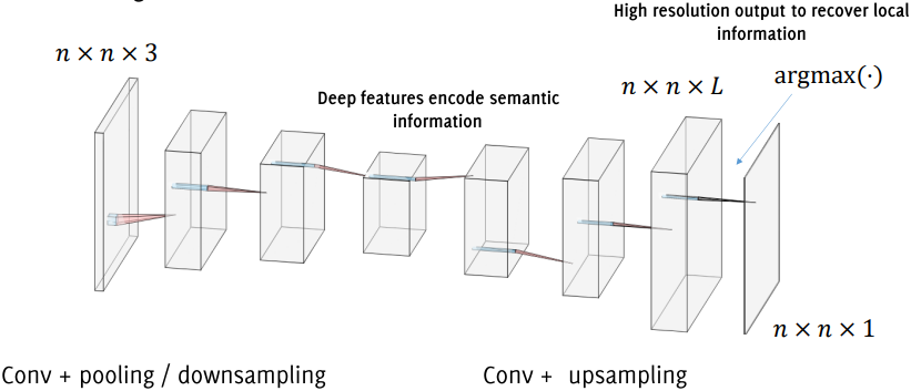
A typical FCN architecture for semantic segmentation has two primary parts:

1. Downsampling Path (Encoding): The initial layers of the network perform convolutions and pooling operations, progressively reducing the spatial resolution of the image while capturing high-level semantic features.

2. Upsampling Path (Decoding): The second part of the network focuses on upsampling these features back to the original image resolution. This phase allows the network to make pixel-wise predictions, ensuring that each pixel is assigned to a class label.

Various upsampling techniques are used to restore spatial resolution, including:

• Nearest Neighbor: This approach duplicates neighboring pixel values, resulting in a simple but somewhat rough upscaling.
• Bed of Nails: This method places non-zero values at regular intervals, filling gaps with zeros to achieve sparse outputs, which are subsequently smoothed by convolutional layers.

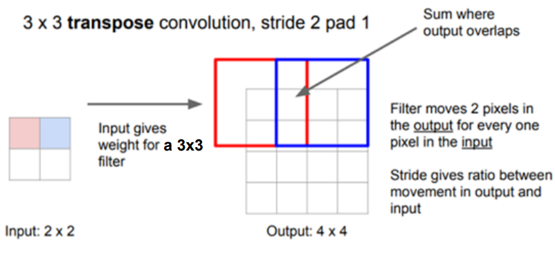
A more sophisticated method, Transpose Convolution (also known as deconvolution or fractional strided convolution), involves reversing the convolution process. Transpose convolution allows learned filters to refine the upsampled outputs, providing a higher degree of control over pixel-wise predictions. While effective, this operation can be computationally intensive.

Loss Function and Optimization

Training an FCN for semantic segmentation typically involves minimizing a loss function that captures the discrepancy between the predicted and ground truth labels at each pixel. The most common approach is to use categorical cross-entropy loss, applied on a per-pixel basis. This loss function calculates the difference between predicted probabilities and the true class labels across all pixels in the image, enabling the network to assess performance at a granular level.

Mathematically, the loss function can be expressed as:

where denotes each pixel in the input image, and represents the pixel-wise loss with respect to the ground truth. In this context, each image or region effectively provides a mini-batch for gradient estimation, contributing to the optimization process.

U-Net: Architecture and Training

The U-Net is a convolutional neural network architecture designed primarily for semantic segmentation tasks, especially in biomedical image analysis. Its structure is characterized by a symmetric “U” shape, which enables precise localization while capturing high-level context. U-Net is composed of two main paths: a contracting path for downsampling, which captures context, and an expansive path for upsampling, which enables precise localization by restoring spatial dimensions. This design makes U-Net particularly effective for tasks requiring high-resolution predictions with fine detail.

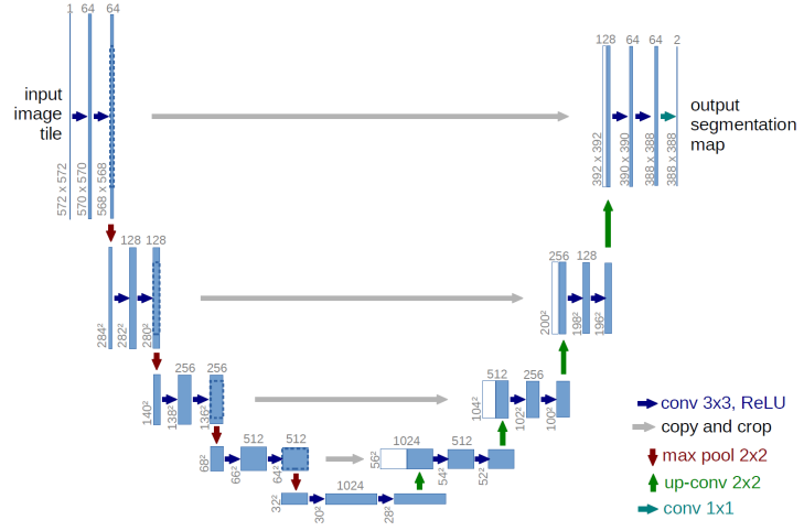
Contracting Path

The contracting path in U-Net performs feature extraction and downsampling, progressively reducing spatial dimensions while increasing the number of feature channels. Each downsampling step consists of two convolutional layers with ReLU activation, followed by max pooling with a stride of 2. The “valid” padding ensures that no padding is applied, resulting in a gradual reduction of the spatial size of the feature maps.

Importantly, at each downsampling step, the number of feature maps is doubled, allowing the network to capture increasingly complex representations of the image content.

Expansive Path

The expansive path is symmetric to the contracting path and serves to reconstruct the spatial resolution of the input image. Each upsampling step consists of a transpose convolution, which doubles the spatial dimensions and halves the number of feature maps. A key feature of U-Net is the skip connections between corresponding layers in the contracting and expansive paths. These connections concatenate high-resolution features from the contracting path with the upsampled features in the expansive path. This fusion of local and global information helps the model achieve both accurate object boundaries and contextual understanding. After each concatenation, the features undergo two convolutional layers with ReLU activation to further refine the output.

The architecture does not use any fully connected layers, making it highly suitable for dense prediction tasks where every pixel needs to be classified. At the network’s top, convolutions are applied to reduce the depth of the feature maps, producing a final output with a specified number of classes.

Key Differences Compared to Previous Architectures

The U-Net introduces a number of innovations compared to earlier segmentation networks, such as the model proposed by Long et al. (2015):

1. Increased Feature Channels in the Upsampling Path: Unlike previous methods, U-Net maintains a high number of feature channels during upsampling, creating a symmetric network structure.
2. Extensive Data Augmentation: U-Net uses aggressive data augmentation techniques, such as elastic deformations, to increase the variability of the training images, improving the network’s robustness and performance on unseen data.

Loss Function and Weighted Training

Training U-Net involves optimizing a weighted loss function to handle class imbalance and improve segmentation accuracy, especially near object borders. The weighted loss function is formulated as follows:

where is a weight assigned to each pixel and is the loss at that pixel, usually defined as cross-entropy loss.

The weighting function is structured to emphasize boundary pixels and address class imbalances:

• : Balances class proportions, accounting for any imbalance in the training set.
• and : Represent the distances from each pixel to the nearest and second-nearest cell boundaries, respectively.

This term highlights pixels near borders, helping the network to distinguish between adjacent objects by assigning higher weights to boundary pixels. Thus, this weighting mechanism improves segmentation performance at object boundaries, which are crucial for tasks like cell segmentation.

Implementing a U-Net Block in Keras

The U-Net architecture can be implemented in Keras by defining each U-Net block as a sequence of convolutional layers, batch normalization, and activation functions. Here’s an example of a U-Net block:

from tensorflow.keras import layers as tfkl
 
def unet_block(input_tensor, filters, kernel_size=3, activation='relu', name=''):
    # First 2D convolution
    x = tfkl.Conv2D(filters, kernel_size=kernel_size, padding='same', name=name+'conv1')(input_tensor)
    x = tfkl.BatchNormalization(name=name+'bn1')(x)  # Optional batch normalization
    x = tfkl.Activation(activation, name=name+'activation1')(x)
    
    # Second 2D convolution
    x = tfkl.Conv2D(filters, kernel_size=kernel_size, padding='same', name=name+'conv2')(x)
    x = tfkl.BatchNormalization(name=name+'bn2')(x)  # Optional batch normalization
    x = tfkl.Activation(activation, name=name+'activation2')(x)
    
    return x

In each block, the concatenation step occurs along the channel dimension, enabling the network to retain detailed spatial information by combining low-level features with high-level context.

Fully Convolutional Networks (FCNs)

Fully Convolutional Networks, or FCNs, are a specialized type of convolutional neural network (CNN) designed to handle input images of varying sizes without requiring a fixed input shape. Traditional CNNs often include fully connected (FC) layers at the end of the architecture to generate a fixed-length output, such as class scores, which necessitates a fixed input size. FCNs eliminate this constraint by replacing fully connected layers with convolutional layers, allowing them to handle images of arbitrary dimensions. This flexibility is essential for dense prediction tasks such as segmentation, where the output size directly correlates with the input size.

Converting Fully Connected Layers to Convolutional Layers

In a typical CNN, convolutional layers can process input images of any size, yielding output feature maps that are reduced in spatial size due to pooling and other downsampling layers. However, once the network reaches a fully connected (FC) layer, the input size must be fixed to match the expected number of neurons. To convert an FC layer to a convolutional one, we reinterpret the weights of the FC layer as a convolution. Specifically, a fully connected layer with neurons and input features can be replaced by a convolutional layer with filters, each having a depth of , effectively generating feature maps without flattening the spatial dimensions.

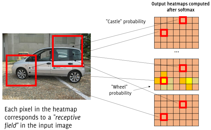
The output of this transformation provides a probability map or class “heatmap” for each category, showing the probability of each class across spatial regions of the image.

Mathematically, the output for a particular neuron in a fully connected layer is computed as:

where are the weights, are the input features, and is the bias. By reshaping these weights into convolutional filters, we obtain a fully convolutional representation that applies these filters across the entire spatial dimensions of the input.

When a classification CNN is converted to an FCN, the model generates a class probability map or heatmap instead of a single class label. Each class is represented as an image of scores, with lower spatial resolution than the original input image. This map indicates the class probabilities for each spatial location, effectively producing localized predictions over the image. This approach is advantageous in tasks like object detection, where spatial information about class presence is crucial.

Migrating a Pretrained Model to an FCN

If we have a pretrained CNN model with fully connected layers, converting it to an FCN involves the following steps:

1. Extract Weights: Retrieve the weights of the fully connected layers.
2. Reshape Weights: Reshape these weights into convolutional filters, with each filter corresponding to a class.
3. Replace Fully Connected Layers: Insert the reshaped convolutional filters into the network as convolutional layers, preserving the spatial dimensions.

This migration enables the model to apply its learned filters across the entire spatial extent of the input, allowing it to process inputs of arbitrary sizes.

FCN in Keras

Below is an example in Keras, where a pretrained CNN model cnn is adapted into an FCN variant cnn2. Here, we assume the fully connected layer we want to replace is layer 7.

# Extract weights from a fully connected layer in the pretrained model
w7, b7 = cnn.layers[7].get_weights()
 
# Reshape the weights to a 1x1 convolutional filter
w7_reshaped = w7.reshape(1, 1, w7.shape[0], w7.shape[1])
 
# Set the reshaped weights to the corresponding convolutional layer in the FCN model
cnn2.layers[7].set_weights([w7_reshaped, b7])

Handling Flatten Layers

Some CNNs contain a flattening layer before reaching the fully connected layers. This flattening step compresses spatial information into a vector, which is incompatible with the FCN structure. To maintain spatial resolution, we replace the flatten layer with a convolutional layer that has the same spatial size as the final activation map before flattening.

An example of this replacement is shown below, assuming that conv4 is the activation map before flattening, and fully_conv_1 represents the replacement layer with matching dimensions:

fully_conv_1 = tfkl.Conv2D(
    filters=256,                 # Number of filters equivalent to the number of FC neurons
    kernel_size=(12, 12),        # Spatial dimensions matching the pre-flattening feature map
    padding='valid',             # Convolution options need to be 'valid' to yield a single response
    activation='relu',
    name='fully_conv_1'
)(conv4)

Defining an FCN Model in Keras

Once all fully connected layers are replaced with convolutional layers, we can define an FCN model that takes inputs of varying spatial dimensions. Below is an example defining the input layer and final output layer for a segmentation task, where the output layer is a convolution that produces class scores:

# Input layer with flexible spatial dimensions
fc_input_shape = (None, None, 3)  # Allow any width and height
input_layer = tfkl.Input(shape=fc_input_shape, name='Input')
 
# Final output layer, predicting scores for each class
output_layer = tfkl.Conv2D(
    filters=output_shape[-1]                   # Number of classes
    kernel_size=(1, 1),
    padding='valid',
    activation='softmax',
    name='fully_conv_2'
)(fully_conv_1)

In this setup, the FCN architecture is capable of generating output predictions for input images of varying sizes. Each convolutional layer in the FCN maintains the same number of parameters as the dense layer it replaces, ensuring a smooth transition from the original CNN while preserving its learned features.

Transitioning from Classification to Semantic Segmentation

Given a pre-trained CNN model for image classification, the challenge is to adapt it into a fully convolutional network (FCN) capable of dense, pixel-wise semantic segmentation on images of arbitrary size. Below are some approaches and solutions to achieve this, progressively refining output resolution and accuracy.

1. Pre-trained CNN Model: Start with a CNN trained for classification. This model has been trained to recognize objects within a fixed image size, typically outputting a single prediction for the entire image.
2. Transfer Learning: Optionally, fine-tune the model weights to align with the segmentation task.
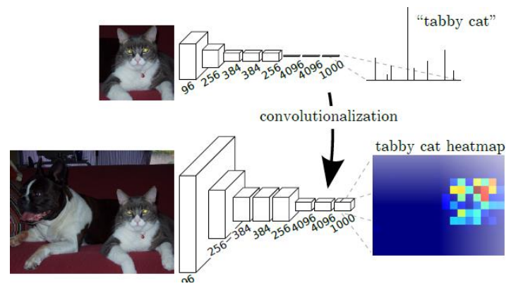
3. Convolutionalization: Convert fully connected layers to convolutions to produce class score heatmaps. This enables us to use the entire image rather than crops for prediction, generating class-specific probability heatmaps.

Standard classification CNNs yield coarse heatmaps after convolutional and pooling layers. These downsampled maps provide broad object localization but lack fine-grained pixel-wise precision. The objective is to adapt the pre-trained model for precise semantic segmentation by creating high-resolution, pixel-wise predictions that maintain spatial accuracy.

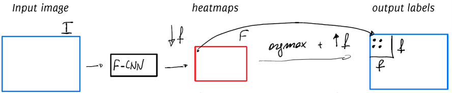
Simple Solution 1: Direct Heatmap Predictions

One option is to apply the low-resolution heatmap directly:

• Receptive Field Assignment: Assign the predicted class label of each heatmap pixel to the corresponding receptive field in the original image. While this method is quick, it results in very coarse segmentation that overlooks smaller details.
• Argmax: Compute the argmax along the class dimension of the heatmap, selecting the class with the highest posterior probability for each pixel region. This approach offers a starting point but lacks the detail required for fine segmentation.

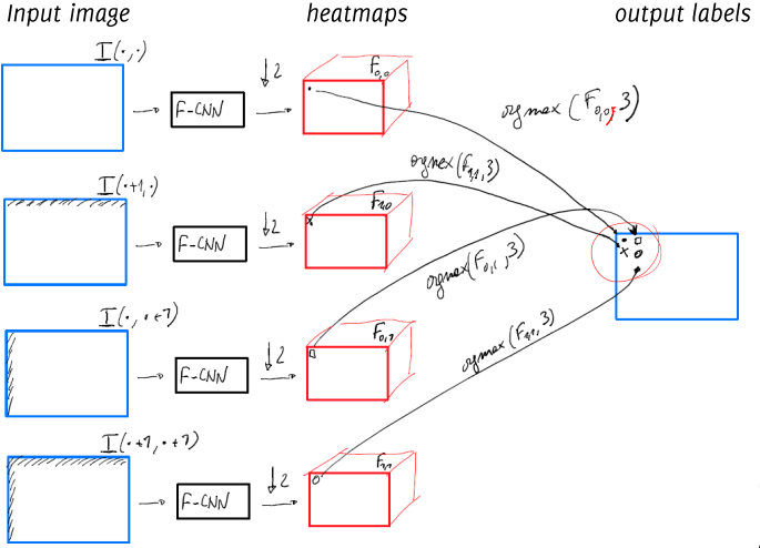
Simple Solution 2: Direct Heatmap Upsampling

This method involves refining the heatmap predictions using shifts to increase resolution:

1. Downsampling Ratio: Assume the input-to-heatmap downsampling ratio is .
2. Shifts and Multiple Heatmaps: For each possible shift where , generate shifted versions of the input image. Compute the heatmap for each shifted version.
3. Mapping and Interleaving: Interleave the results from these heatmaps so that each covers a portion of the input image, yielding a high-resolution output.

Using atrous (dilated) convolutions can replicate the shift-and-stitch effect more efficiently. Here, filters are dilated to cover a broader region without downsampling, allowing the network to preserve resolution while maintaining spatial coverage.

An alternative method avoids explicit shifting:

• Remove Strides: Remove strides in pooling or convolution layers, effectively computing outputs for all shifted versions in one pass.
• Rarefy Filters: For the next convolutional layer, upsample filters and add zero-padding to mimic the effects of dilated filters.
• Repeat Process: Apply this modification to each subsampling layer to maintain full spatial coverage.

The Shift-and-Stitch method offers several benefits. It leverages the full depth and learned features of the network, ensuring that the model’s capabilities are fully utilized. Additionally, it efficiently upsamples outputs, providing a higher resolution prediction. However, the method’s rigidity in application can pose challenges, as it may not adapt well to all scenarios.

Solution 3: Learning Data-Driven Upsampling in an FC-CNN

In FCNs, data-driven upsampling is applied to the coarse feature maps to achieve pixel-dense outputs. Key steps include:

1. Bilinear Initialization: Initialize upsampling layers with bilinear interpolation filters. This initial configuration provides a basic upsampled output before further refinement during training.
2. Upsampling Filters: Use transposed convolutions (fractional striding) to perform upsampling by learning filters that produce smooth, detailed predictions.
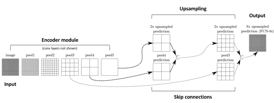
3. Skip Connections: Introduce skip connections to merge features from both coarse and fine layers, which helps the model make localized predictions that preserve global structure.

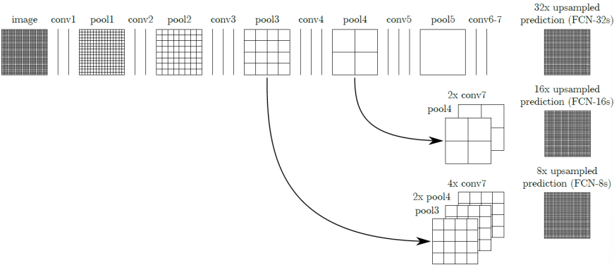
Each FCN variant refines predictions at progressively higher resolutions:

• FCN-32s: Predicts segmentation at a coarse resolution.
• FCN-16s: Initialized with FCN-32s, combines finer details.
• FCN-8s: Initialized with FCN-16s, achieves the highest resolution.

Each of these variants benefits from transferring weights from lower-resolution networks, improving performance while retaining the original classification features.

Fully Convolutional Networks (FCNs) offer several advantages for segmentation tasks. One of the primary benefits is their ability to process the entire image at once, enabling end-to-end training and inference. This approach not only simplifies the training process but also ensures that the model can leverage the full context of the image for more accurate predictions.

Another significant advantage of FCNs is their compatibility with transfer learning. FCNs can be initialized with pre-trained models and fine-tuned for segmentation tasks. This adaptability is particularly useful when working with smaller datasets, as it allows the model to benefit from the knowledge gained from larger, pre-trained datasets.

FCNs are also known for their ability to produce detailed, high-quality segmentations. By learning upsampling filters and incorporating skip connections, FCNs can maintain spatial accuracy and generate precise segmentation maps. This capability is crucial for applications that require fine-grained segmentation results.

Finally, FCNs can handle input images of any size, thanks to their fully convolutional nature. This flexibility means that FCNs can produce segmentation maps with resolutions proportional to the input, making them suitable for a wide range of image sizes and resolutions.

Patch-wise Training vs. Full-image Training

Semantic segmentation models aim to label each pixel in an image according to its class. Training these models typically follows either a patch-wise approach or a full-image approach. Here’s a breakdown of both methods, along with their strengths and limitations.

Patch-based Training

In patch-based training, the segmentation model learns from small patches extracted from annotated images.

Algorithm

1. Prepare Training Set: Gather patches from annotated images.
2. Label Assignment: Each patch receives the label of its central pixel.
3. Train Classification Model: A CNN is trained for patch classification, which can be done from scratch or by fine-tuning a pre-trained model.
4. Convolutionalization: Once trained, fully connected (FC) layers are converted to convolutional layers, and an upsampling mechanism is designed and trained for full-image segmentation.

Loss Function: The training minimizes the classification loss over a mini-batch of patches:

where is a patch in batch .

Advantages	Limitations
Patch-wise training allows for more control over mini-batches, which can help in handling class imbalance by resampling patches from underrepresented classes.	Redundant Computations: Many patches overlap, leading to repeated calculations on shared regions, which makes patch-wise training inefficient.
	Local Context Only: The network processes each patch independently, which limits its ability to learn global image context.

Full-image Training

Full-image training uses the entire annotated image as input, allowing the network to learn from all pixels simultaneously.

Algorithm

1. End-to-End Training: The CNN is trained in an end-to-end manner to predict the segmented output directly for each pixel.
2. Efficient Convolutional Processing: Fully convolutional training processes the whole image at once, computing gradients for all pixels in a region simultaneously, leveraging shared convolutional calculations.
3. Direct Segmentation Loss: The model learns to minimize segmentation loss over all pixels in :

Full-image training offers several benefits. It enhances efficiency by calculating convolutions once for the entire image, thereby reducing redundancy. This approach also allows the model to capture and leverage global context across the whole image, which is crucial for accurate segmentation. Additionally, full-image training streamlines the process by directly training the model for segmentation, avoiding the need for a two-step process where a classification model is first trained and then converted for segmentation.

Limitations of Full-image Training and Potential Solutions

1. Non-random Mini-batches: Unlike patch-based training, full-image training does not use randomly assembled batches, which can limit the stochastic nature of the training process. To counteract this:

   • Random Masking: Introduce a binary random mask to randomly select pixels:
   • This adds an element of randomness, making the estimated loss more stochastic.

2. Class Imbalance: In patch-based training, underrepresented classes can be resampled more frequently. For full-image training, this is not directly feasible, so instead:

   • Weighted Loss: Use a weighted loss function where weights depend on the true class of each pixel:
   • This allows the model to focus more on less common classes by increasing their influence in the loss calculation.

Summary of Patch-based vs. Full-image Training

Aspect	Patch-based Training	Full-image Training
Input	Small image patches	Whole image
Efficiency	Lower, redundant convolutions	Higher, fewer redundant calculations
Global Context	Limited	Entire image context
Class Imbalance	Addressed by patch resampling	Addressed by weighted loss
Batch Stochasticity	High	Lower (addressed by random masking)
Computation	Multiple passes over overlapping regions	Single pass with shared convolutions

---

References

• Google Colab - From CNN to FullyCNN