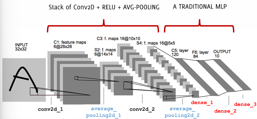
LeNet-5, developed by Yann LeCun and colleagues in 1998, was a pioneering convolutional neural network architecture primarily designed for character recognition tasks, such as handwritten digit classification in the MNIST dataset. The architecture of LeNet-5 is structured as a stack of alternating layers, combining Conv2D layers, ReLU activation functions, and average pooling layers, followed by a traditional multi-layer perceptron (MLP) to connect the convolutional layers with the output layer.
The Conv2D layers play the role of automatically learning feature hierarchies in the input images, while average pooling serves to reduce spatial dimensions, promoting generalization and computational efficiency. Although simple by modern standards, LeNet-5 successfully demonstrated the viability of convolutional networks for real-world applications, laying down the foundational principles of convolutional processing and hierarchical feature extraction that would be extended in later architectures.
AlexNet (2012)
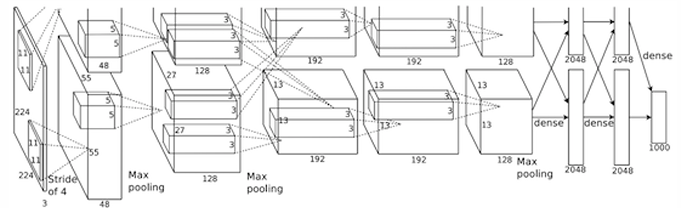
AlexNet, introduced by Alex Krizhevsky, Ilya Sutskever, and Geoffrey Hinton in 2012, marked a turning point in computer vision and deep learning. Winning the ImageNet Large Scale Visual Recognition Challenge (ILSVRC) in 2012, this network architecture outperformed existing models by a large margin and drew widespread attention to the power of deep learning in complex image classification tasks. Building on the basic structure of LeNet-5, AlexNet adopts a similar convolutional stack but significantly expands the depth and complexity of the network.
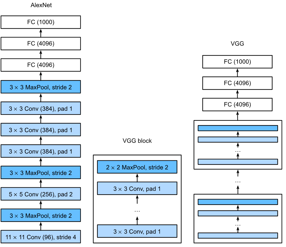
The architecture of AlexNet consists of five convolutional layers, with the initial layers using large filter sizes, notably and . These convolutional layers are followed by three fully connected layers (MLP), which together serve to increase the network’s capacity to learn complex features from the input images. The input to AlexNet is of size (RGB channels), although the original paper references , which highlights a slight discrepancy that does not affect the network’s performance. The model contains approximately 60 million parameters, with the vast majority concentrated in the fully connected layers: 3.7 million parameters (about 6%) are in the convolutional layers, and the remaining 58.6 million (roughly 94%) are within the fully connected layers.
To enhance performance and combat overfitting, AlexNet introduced several critical innovations in deep learning:
ReLU Activation:
Unlike traditional activation functions such as tanh, AlexNet employed the Rectified Linear Unit (ReLU) function, which not only accelerates convergence during training but also helps in mitigating the vanishing gradient problem.
Dropout Regularization:
To prevent overfitting in the fully connected layers, AlexNet used dropout with a probability of , effectively randomly “dropping out” neurons during training to force the network to learn redundant representations and improve generalization.
Weight Decay and Norm Layers:
These techniques were also implemented to further regularize the model, although some (like normalization layers) are no longer commonly used in modern CNN architectures.
Max Pooling:
AlexNet replaces the average pooling used in LeNet-5 with max pooling, which not only enhances spatial invariance but also selectively preserves high activations, believed to correspond to the most important features in an image.
The first convolutional layer of AlexNet uses 96 filters of size with a stride of 4, producing output volumes of size . The network was initially trained across two GTX 580 GPUs with 1.5 GB of memory each, splitting the model in such a way that each GPU handled different parts of the network. This setup allowed for parallel computation of feature maps, and the two GPUs’ outputs were merged in the final layers. AlexNet was trained over 90 epochs, taking about five to six days to complete on this hardware setup. Notably, AlexNet’s success was further enhanced by an ensemble of seven models, which reduced the top-5 error rate on the ImageNet dataset from 18.2% to 15.4%.
VGG16 (2014)
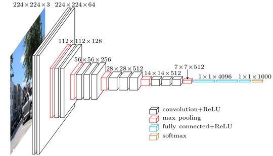
Introduced by the Visual Geometry Group at Oxford in 2014, VGG16 represents a significant evolution from earlier CNN architectures such as AlexNet. While AlexNet popularized the use of deep neural networks in image classification, VGG16 extended this approach by increasing network depth and simplifying filter sizes, introducing a more structured and scalable design for CNNs. This deeper architecture relies on the use of small, uniform filters throughout the network, achieving both high performance and efficient parameterization.
The VGG16 model, with 138 million parameters, is designed to handle input images of size , which is similar to the input size for AlexNet. In terms of performance, VGG16 achieved first place in the localization track and second place in the classification track of the 2014 ImageNet Challenge. This achievement showcased its superior feature extraction capabilities for complex image recognition tasks, establishing VGG16 as a powerful model for large-scale image classification.
Architectural Design and Depth Analysis
One of the main contributions of the VGG16 paper was its systematic study of network depth and its impact on performance. The design philosophy behind VGG16 was to “fix other parameters of the architecture and steadily increase the depth of the network by adding more convolutional layers.” To make this feasible without an explosive increase in computational cost, VGG16 employs small convolution filters in each layer, instead of larger filter sizes commonly used in earlier networks. By stacking multiple convolutional layers in sequence, VGG16 achieves a large receptive field effectively, without the need for large filters.
Using three layers of convolutions provides a receptive field equivalent to a filter but with fewer parameters and more nonlinear activation points:
3 layers
1 layer
receptive filed
number of filter weights
number of nonlinearities
Receptive Field: Both a single filter and a sequence of three filters have a receptive field of .
Parameter Efficiency: A single filter requires 49 weights, whereas three filters require only 27 weights (3 filters, each with 9 weights).
Nonlinearity: Three stacked layers provide three activation functions (e.g., ReLU) compared to only one with a single filter, introducing more opportunities for the network to learn complex, nonlinear features.
VGG16 comprises five blocks of convolutional layers, where each block is followed by a max-pooling layer to reduce spatial dimensions, promoting computational efficiency. The sequence within each block generally follows a structure of two or three convolutions, all employing ReLU activations:
Block 1: Two convolutional layers with 64 filters, followed by a max-pooling layer.
Block 2: Two convolutional layers with 128 filters, followed by max-pooling.
Block 3: Three convolutional layers with 256 filters, followed by max-pooling.
Block 4: Three convolutional layers with 512 filters, followed by max-pooling.
Block 5: Three convolutional layers with 512 filters, followed by max-pooling.
Following the convolutional blocks, the output is flattened and passed through three fully connected (FC) layers, two with 4096 units each, and the final layer with 1000 units, corresponding to the 1000 classes in ImageNet. This arrangement places 89% of the network’s parameters in the FC layers, while the convolutional layers account for the remaining 11%.
Training VGG16 requires substantial computational resources, particularly in terms of memory. The model’s extensive depth and large number of parameters result in high memory consumption, which poses challenges during training:
Memory Requirements: Forward and backward passes demand around 100 MB per image for storing activations, doubling to 200 MB per image during training due to the need to store gradients and intermediate activations.
Parameter Storage: With 138 million parameters, VGG16 requires careful optimization and resource allocation, making it challenging to train on standard consumer-grade GPUs without memory issues.
Network in Network (NiN, 2014)
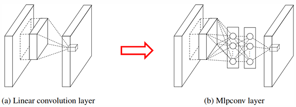
The Network in Network (NiN) model, introduced in 2014, innovates on traditional CNN structures by employing MLPconv layers—a sequence of fully connected (FC) layers with ReLU activations in place of standard convolutional layers. By applying these fully connected layers in a sliding window fashion across the entire image, NiN achieves more complex functional approximations than the simple linear transformations typical in traditional convolutional layers. In contrast to standard convolutions that use linear filters, MLPconv layers enable the network to learn nonlinear transformations at every spatial location, resulting in a more expressive model with enhanced feature extraction capabilities.
In NiN, however, each convolutional output can be processed by a multi-layer perceptron (MLP), leading to a more complex transformation like:
This setup allows for additional layers of ReLU activations within each convolution, offering greater nonlinearity and enhancing the network’s ability to model intricate patterns in data.
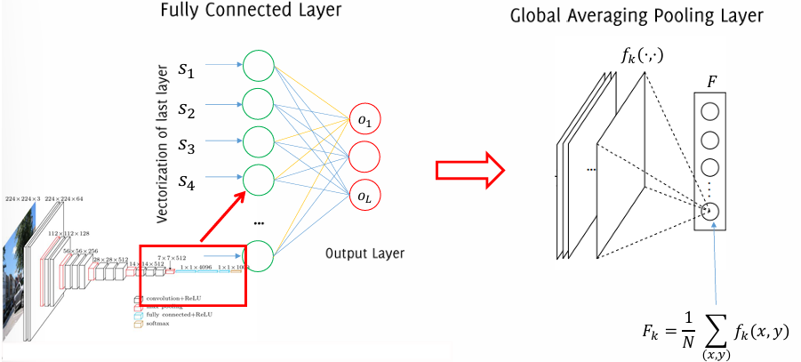
Introduction of Global Average Pooling (GAP)
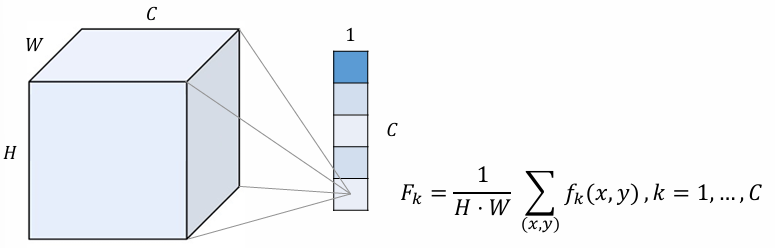
Another innovative feature of NiN is the Global Average Pooling (GAP) layer. Unlike traditional CNNs that often use fully connected (FC) layers at the network’s end for classification, NiN replaces the FC layer with a GAP layer. In this layer, the average value of each feature map is computed, effectively summarizing each map into a single value without adding any additional parameters. This approach reduces the risk of overfitting, as FC layers can introduce a large number of parameters.
The GAP layer operates similarly to a block-diagonal matrix that averages spatial values across each feature map. This is fundamentally different from an MLP, which involves a dense matrix multiplication. Some key benefits of GAP include:
Reduced Overfitting: The GAP layer avoids the need for large FC layers, which can lead to overfitting due to their high parameter count.
Structural Regularization: GAP serves as a form of regularization, reducing the network’s complexity while retaining classification performance.
Spatial Invariance: Since GAP performs a global operation, it is less sensitive to spatial shifts in input images, enhancing the model’s robustness to shifted inputs.
Interpretable Mapping: GAP creates a more interpretable model by establishing a direct relationship between the feature maps and the output classes, which can be useful for tasks such as localization.
In NiN, the GAP layer is used as follows:
The final fully connected layer is removed.
A GAP layer is added in its place.
Classification is performed with a softmax layer after the GAP layer.
Importantly, the number of feature maps must correspond to the number of output classes to ensure that the GAP layer produces an output compatible with the softmax layer. If the number of channels and classes differs, an additional hidden layer can adjust the feature dimensions.
The use of GAP, along with MLPconv layers, provides NiN with the following advantages:
Parameter Efficiency: Without the need for an FC layer at the end, NiN has a smaller parameter count, making it less prone to overfitting.
Enhanced Feature Learning: MLPconv layers allow the network to capture more complex relationships within feature maps.
Shift Invariance: GAP increases the model’s robustness to spatial transformations of input images, enhancing generalization.
The NiN architecture achieves state-of-the-art performance on smaller datasets, such as CIFAR-10, CIFAR-100, SVHN, and MNIST, largely due to the overfitting resistance provided by GAP.
GAP as a Structural Regularizer
GAP’s regularization effect is evident when comparing error rates between models with and without GAP:
Method
Testing Error
MLPconv + Fully Connected
11.59%
MLPconv + Fully Connected + Dropout
10.88%
MLPconv + Global Averaging Pooling
10.41%
In GAP, a single value per channel is kept by performing an average or max pooling across spatial dimensions.
For example, in Keras, a GAP layer is implemented as:
gap = tfkl.GlobalAveragePooling2D(name='gap')(x)
GAP is particularly useful for achieving shift invariance. In a CNN without GAP, shifting an image may lead to incorrect classifications, as the flattened fully connected layer’s weights might not capture spatial shifts. By applying GAP, shifted images produce similar feature map summaries, allowing the network to generalize better.
Example
To illustrate the advantages of GAP, consider two CNN architectures trained on a zero-padded MNIST dataset:
CNN with Flattening: This architecture includes a traditional CNN with a flattening layer before the final fully connected classifier.
CNN with GAP: Here, the same CNN structure is used, but GAP is applied before classification.
Both models are trained on centered images and tested on both centered and shifted test sets. The CNN with GAP shows improved performance on shifted test images due to its spatial invariance, demonstrating GAP’s effectiveness as a structural regularizer.
When designing deep neural networks, the straightforward approach to improving performance is to increase their size, either by making them deeper or wider. However, this approach has drawbacks:
Increased Overfitting: Larger networks often have more parameters, making them more prone to overfitting, especially with limited data.
Higher Computational Demand: Bigger networks require significantly more computational resources, which can become impractical in real-world applications.
Moreover, features in images may appear at different scales, making it difficult to determine the optimal filter size for capturing relevant features.
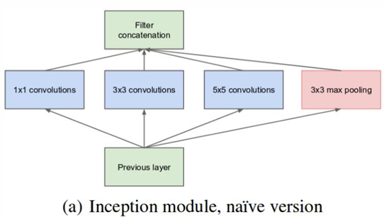
The Inception module addresses these challenges by using parallel convolution operations of multiple filter sizes (e.g., , , and ). Each filter size captures features at different scales, and the outputs are concatenated along the channel dimension to form a richer, multi-scale feature representation.
The module includes:
Convolutions: Capture fine details and are computationally inexpensive.
and Convolutions: Capture larger features and patterns in the data.
Max Pooling: Adds more spatial information.
By concatenating these activations, the network preserves spatial dimensions while greatly expanding depth, leading to a more expressive feature representation. Zero padding is used for convolutional filters, and fractional strides are employed for pooling operations to ensure that spatial dimensions remain consistent across the layers.
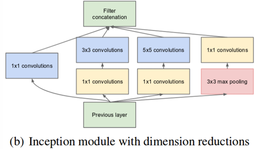
Addressing Computation Costs with Bottleneck Layers
A direct use of large filter sizes on deep input tensors can lead to computational inefficiency. For example, using multiple filters without dimensionality reduction can require around 854 million operations per layer. To mitigate this, 1x1 convolutions, also known as bottleneck layers, are introduced before the larger and convolutions to reduce the number of channels, thus significantly decreasing computation costs. This approach not only reduces the number of required operations to approximately 358 million but also increases the number of nonlinearities within the network, making it more powerful without a massive computational burden.
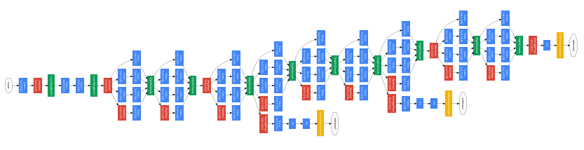
GoogLeNet Architecture
GoogLeNet is built by stacking Inception modules, creating a network that is deep yet efficient. Key characteristics of GoogLeNet include:
Parallel Processing: Instead of sequential layers, GoogLeNet features multiple branches within each Inception module, processing the input in parallel.
Layer Structure: The network begins with two blocks of standard convolution and pooling layers, followed by a series of nine Inception modules.
Global Average Pooling (GAP): Replaces fully connected layers at the end of the network, reducing the number of parameters and enhancing shift invariance. The network’s final classification layer is a softmax applied after GAP.
Auxiliary Classifiers: To address the dying neuron problem (where neurons stop updating during training), GoogLeNet introduces two auxiliary classifiers in intermediate layers. These classifiers compute an auxiliary loss, encouraging intermediate layers to produce meaningful feature representations and aiding in gradient flow. These auxiliary heads are used only during training and are removed during inference.
Inception Module Implementation Example in Keras
The following code demonstrates how to implement an Inception module in Keras:
# Define input x x = tfkl.MaxPooling2D(name='mp')(x) # Branch with 1x1 convolutionx1 = tfkl.Conv2D(32, kernel_size=1, padding='same', activation='relu', name='conv_1_1')(x) # Branch with 3x3 convolutionx2 = tfkl.Conv2D(64, kernel_size=1, padding='same', activation='relu', name='conv_2_1')(x) # Branch with max poolingx4 = tfkl.MaxPooling2D((3,3), strides=(1,1), padding='same', name='mp_4_1')(x) # Concatenate along the last axis to combine branchesy = tfkl.Concatenate(axis=-1, name='concat')([x1, x2, x4])
This setup ensures that spatial dimensions are preserved across the layers due to padding and appropriate stride choices.
Model Summary of GoogLeNet
A typical GoogLeNet model includes 27 layers (counting pooling layers) with around 5 million parameters, which is considerably efficient given its depth and performance.
The Inception module allows for a deep, multi-scale analysis of input data while controlling computation and memory costs. Its benefits include:
Multi-Scale Feature Extraction: By combining different convolutional filters, the Inception module captures patterns across multiple spatial scales in the input.
Efficient Computation: Bottleneck layers and parallel processing ensure efficient use of computational resources.
Reduced Parameter Count: With approximately 5 million parameters, GoogLeNet avoids the overfitting issues associated with larger fully connected networks.
Enhanced Gradient Flow: Auxiliary classifiers help mitigate vanishing gradients by providing additional gradient signals during training.
ResNet (2015): Residual Networks
ResNet, introduced in 2015, brought a breakthrough in designing very deep neural networks. It achieved remarkable performance, including a 3.57% top-5 classification error on the 2015 ImageNet ILSVRC challenge, surpassing human-level performance and winning both the classification and localization tasks.
With a depth of up to 152 layers on ImageNet and 1202 layers on CIFAR, ResNet enabled the successful training of extremely deep networks. Prior to ResNet, increasing network depth often did not improve performance because very deep networks were challenging to optimize. Specifically, empirical observations showed that adding layers increased both training and test errors, indicating issues beyond overfitting—namely, the vanishing/exploding gradient problem that made gradient-based optimization ineffective in very deep architectures.
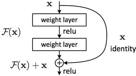
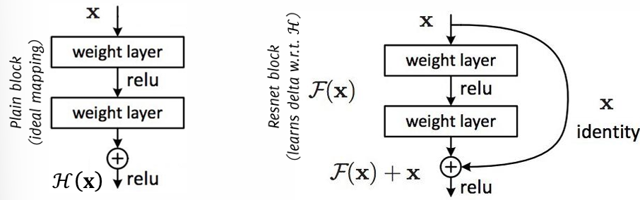
ResNet introduced the identity shortcut connection, or “skip connection,” to address these issues. The main idea is to add a direct connection that bypasses a few layers within each block, allowing the network to pass information without modification. This approach helps mitigate the vanishing gradient problem and stabilizes training in deep architectures by enabling gradient flow across layers.
Key points of identity shortcuts:
No Additional Parameters: Skip connections don’t add parameters or increase computational overhead.
Information Propagation: If the preceding layers are optimal, the weights can approach zero, allowing information to propagate through the identity mapping, requiring the network to learn only incremental changes.
Easier to Train: Instead of learning the entire mapping , the network learns a residual function , which is generally easier to optimize in deep networks.
The network can focus on learning a residual function that “improves” over a simple identity function, thus becoming more efficient at learning subtle differences as the depth increases. This residual learning framework is especially powerful for training very deep networks.
ResNet Architecture
ResNet is structured as a stack of these residual blocks, each containing:
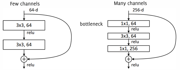
Two Convolutional Layers with ReLU Activations: The layers within the block use convolutions (typically ) with a stride of 1 to maintain the spatial dimensions.
Skip Connection: After the convolutions, the input is added to the output of the final convolution in the block, and a non-linearity (e.g., ReLU) is applied after the addition. This helps retain information and avoid the problem of the network failing to learn identity mappings.
Pooling and Filter Doubling: Outside the residual blocks, ResNet reduces the spatial dimensions with convolutions that use a stride of 2 and doubles the number of filters to increase feature depth progressively.
Global Average Pooling (GAP): Instead of using fully connected layers, ResNet uses GAP before the final softmax, reducing the number of parameters and overfitting risk.
In ResNet architectures with more than 50 layers, bottleneck layers ( convolutions) are used within residual blocks to reduce the number of channels before the primary convolutions. This reduces the network’s depth in each block and significantly cuts computational requirements, similar to the bottleneck layers in Inception modules.
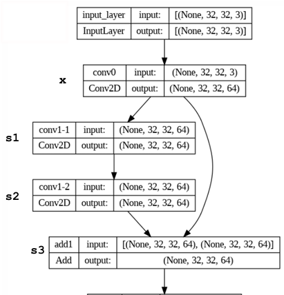
ResNet Block Implementation in Keras
The following code demonstrates how to implement a residual block in Keras:
padding='same' ensures that the spatial dimensions remain constant within the residual block.
Non-linearity after addition: The ReLU activation is applied after the addition of the skip connection, which helps in learning more complex mappings.
Spatial reduction occurs only outside the residual block, ensuring the skip connection inputs and outputs have matching dimensions.
Key Benefits of ResNet
The identity shortcut connection and residual learning framework allow ResNet to efficiently learn in very deep architectures, providing:
Enhanced Gradient Flow: The shortcut connections enable gradients to flow directly through the network, helping mitigate vanishing gradients.
Simplified Learning: Instead of learning full mappings, ResNet learns small, incremental changes (residuals) over identity mappings.
Lower Error Rates: ResNet achieves lower error rates on ImageNet and CIFAR, particularly with very deep networks, due to its stability in optimization.
Efficient Design: By using bottleneck layers and replacing fully connected layers with GAP, ResNet minimizes computational cost without sacrificing performance.
MobileNet (2017): Efficient Networks for Mobile Applications
MobileNet was designed specifically to address the challenges of deploying neural networks on mobile devices. The key issues it aimed to solve were:
High Parameter Count: Standard convolutional layers typically require a large number of parameters, which increases memory requirements.
Computational Complexity: Traditional convolutional layers demand substantial computation, which is limiting for devices with lower processing power, like mobile devices.
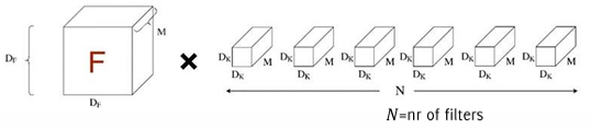
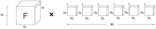
In a standard 2D convolution: each filter combines information across all input channels, effectively learning complex spatial and depth features in one operation. The computational cost for a convolutional layer with filter size , input with channels, output size , and filters is:
To make this computation more efficient, MobileNet employs depth-wise separable convolutions.
Depth-wise separable convolutions split a standard convolution into two smaller, more efficient operations:
Depth-Wise Convolution:
A separate convolution operation is performed on each input channel independently.
This layer learns spatial features within each channel but does not combine information across channels.
Computational cost:
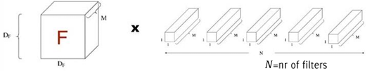
Point-Wise Convolution:
After the depth-wise convolution, a 1x1 convolution is applied across all output channels, combining them into filters.
This step mixes the information across channels without performing further spatial operations.
Computational cost:
The overall computational cost of a layer with depth-wise separable convolution using filters is:
Compared to a standard convolutional layer, depth-wise separable convolution offers significant computational savings. The ratio of computational cost for depth-wise separable convolution to traditional convolution is:
When both (the number of filters) and (the filter size) are large, this fraction is small, indicating substantial savings in computational load and memory usage.