Computer vision is a dynamic interdisciplinary field that focuses on enabling computers to interpret and understand digital images and videos.
By leveraging algorithms and machine learning techniques, researchers have made significant advancements in this domain over the past few years, particularly in training computers to recognize and classify objects within images with remarkable accuracy. This capability is commonly referred to as image classification, which encompasses several key components.
One critical aspect of image classification is object detection, which involves identifying the presence of various objects within an image and determining their specific locations. This process often utilizes Convolutional Neural Networks (CNNs) and other deep learning models that are trained on extensive datasets, allowing the system to learn and generalize from examples. The effectiveness of these models hinges on their ability to discern features and patterns that distinguish different objects, thereby improving recognition rates.
Another important element of image classification is pose estimation, which refers to the process of determining the position and orientation of objects in an image. Accurate pose estimation is vital for applications such as augmented reality and robotic manipulation, where understanding an object’s spatial configuration is essential for interaction and integration with the surrounding environment. Techniques for pose estimation often involve advanced algorithms that analyze key points or landmarks on objects to infer their orientation.
Finally, image captioning is a fascinating aspect of computer vision that involves generating textual descriptions of images. This task combines image processing with Natural Language Processing (NLP) to produce coherent and contextually relevant captions. By utilizing deep learning models trained on paired datasets of images and their corresponding descriptions, systems can learn to articulate the content of an image effectively, paving the way for applications in accessibility, content management, and social media.
Digital Images
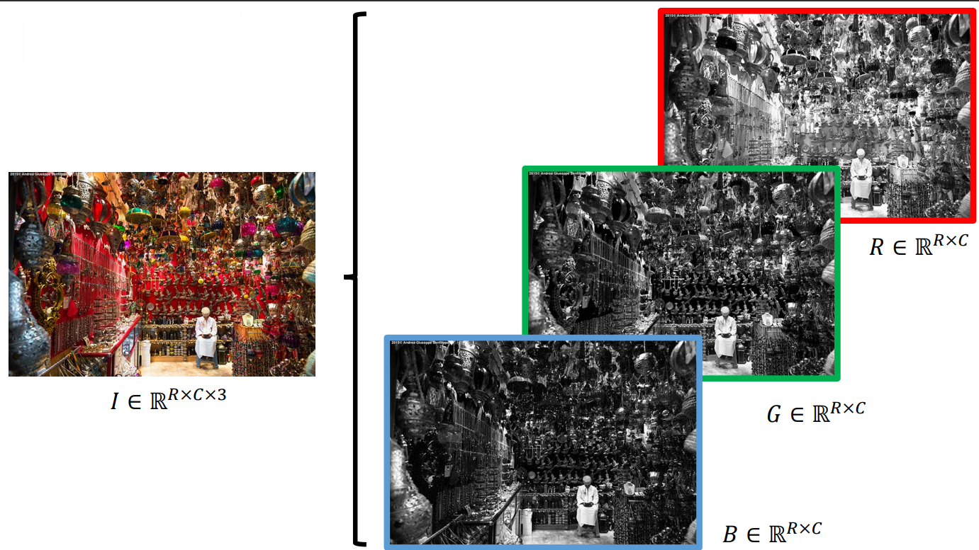
Digital images are composed of small units called pixels, which represent the fundamental building blocks of the image. Each pixel contains information about color, typically represented by a combination of red, green, and blue (RGB) values. These values are encoded using 1 byte (8 bits) per color channel, meaning each pixel’s color can be described using 256 possible intensity levels for red, green, and blue, ranging from 0 to 255.
Definition
Mathematically, a digital image can be represented as a matrix:
where , , and represent the intensity of the red, green, and blue channels for each pixel, and refers to the resolution of the image (i.e., the number of rows and columns of pixels). The color of each pixel is determined by the combined intensities of these three channels.
is the intensity of red (between 0 and 255)
is the intensity of green (between 0 and 255)
is the intensity of blue (between 0 and 255)
Since each color channel is encoded using 8 bits, the total number of distinct colors that can be represented by a pixel is , or approximately million colors. For high-resolution images the uncompressed size of the image can be quite large: for instance, an image of 20 megapixels would require about 60 megabytes of storage (20 megabytes for each color channel, multiplied by 3 channels). This is why image compression formats, such as JPEG, are commonly used to reduce the file size for easier storage and processing.
However, in the context of neural networks, especially during tasks such as training models, images are typically processed at their full resolution. This ensures that no information is lost due to compression, which could impact the performance of algorithms designed to classify or analyze images.
In programming, libraries like skimage in Python allow users to read and manipulate image data directly. For example, the following Python code extracts the red, green, and blue channels from an image:
from skimage.io import imread# Read the imageI = imread('bazar.jpg')# Extract the color channels R = I[:, :, 0]G = I[:, :, 1]B = I[:, :, 2]
A similar operation can be performed in MATLAB:
R = I(:, :, 1);G = I(:, :, 2);B = I(:, :, 3);
When images are loaded into memory, they occupy more space than their compressed versions stored on disk, especially in formats like JPEG. This increased memory usage must be considered when designing algorithms, particularly for deep learning tasks.
Videos
A video is essentially a sequence of images, or frames, displayed in rapid succession to give the illusion of motion. Each frame can be represented by a matrix . For a video consisting of frames, the overall data representation can be described as:
This can be demonstrated in Python:
print(V.shape) # (144, 180, 3, 30)
In this example, the video has 144 rows, 180 columns, 3 color channels, and 30 frames. The total number of pixel values in this video would be , representing the pixel intensities, which amounts to around 388 KB of data (if each pixel value is stored using 1 byte).
However, as video resolution increases, so does the size of each frame. For example, one frame in full HD resolution (1920x1080 pixels) would require approximately 6.22 MB of storage. A single second of video at 24 frames per second (fps) would consume around 186.6 MB of storage.
Given the large size of video data, compression is essential for practical storage and transmission. Video compression algorithms (such as those used in formats like H.264 or HEVC) take advantage of the high redundancy in video data to significantly reduce file sizes while maintaining quality.
Local (Spatial) Transformations
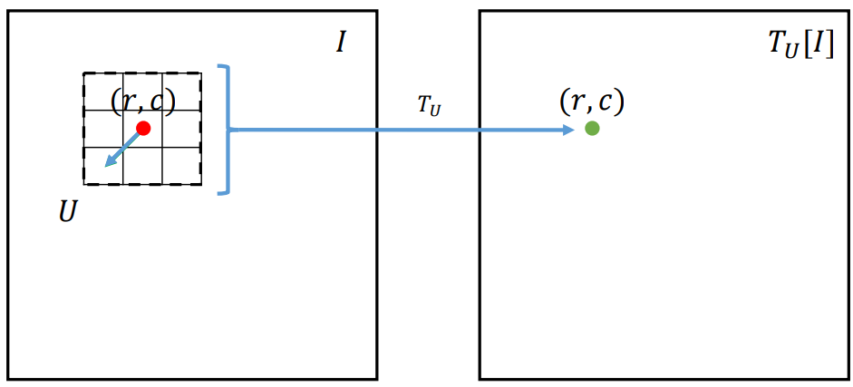
Local spatial transformations involve applying an operation to a pixel in an image based on the pixel values in its surrounding neighborhood. One such transformation is correlation, which is particularly important in image processing tasks like filtering, edge detection, and template matching.
Definition
In a general spatial transformation, each pixel in the output image is computed from the input image , by a transformation function , that processes the local neighborhood around the pixel :
is the input image.
is the output image.
defines the neighborhood around the pixel , often a square region like a or grid.
or is the transformation function that computes the output based on the values in .
The output at each pixel depends on the intensities of pixels in the neighborhood, described by , where is a displacement vector relative to .
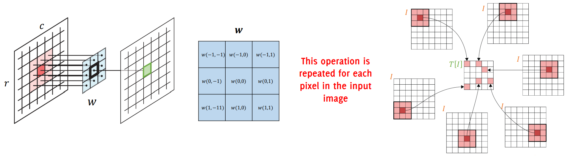
Space-invariant transformations mean the same operation is applied to every pixel in the image, independent of its location. Additionally, transformations can be either linear or nonlinear. A linear transformation implies that the output is a linear combination of the neighboring pixel values.
A local linear filter is a spatial transformation where the output at each pixel is computed as a weighted sum of the pixel values in its neighborhood:
where, are the filter weights, which define how much each neighboring pixel contributes to the output. These weights form a matrix, often referred to as a filter or kernel. The filter (or kernel) fully defines the transformation by determining the relative importance of each pixel in the neighborhood.
Correlation
In the context of image processing, correlation measures the similarity between a filter (or template) and the region of the image it is applied to.
Definition
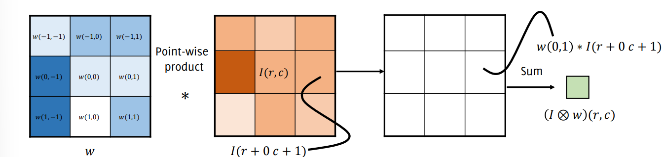
The correlation between an image and a filter is defined as:
In this equation:
The filter (or kernel) is of size , which defines the neighborhood.
The sum is performed over all neighboring pixels within the neighborhood, where controls the window size.
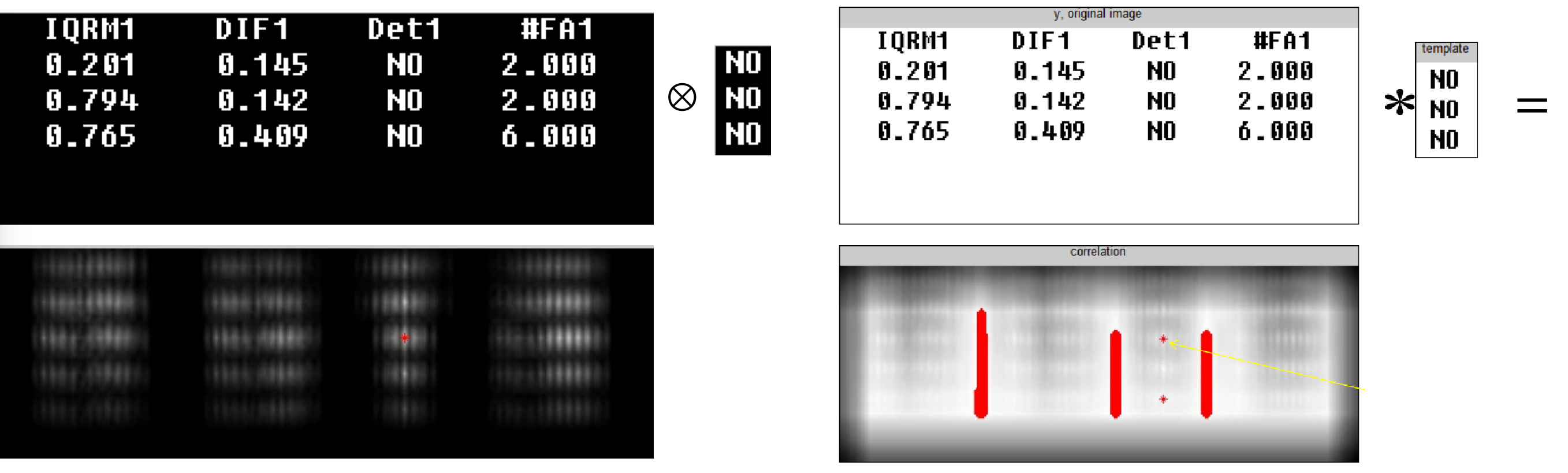
This operation slides the filter across the image, and at each position , the weighted sum of the pixel values is calculated to produce the output. Correlation is widely used in tasks like template matching, where a small template is compared to different regions of an image to find areas of high similarity.
Python example
A simple example of correlation for template matching can be:
acc = 0for i in np.arange(template_height): for j in np.arange(template_width): acc += image[y + i, x + j] * template[i, j]image[x + template_height // 2, y + template_width // 2] = acc
This code computes the correlation at each position by summing the element-wise product of the template and the corresponding pixels in the image.
For binary images, where each pixel is either black (0) or white (1), correlation simplifies significantly:
If the filter and the image match exactly (i.e., the same value at each pixel), the output is 1.
If the filter and image are similar but not identical, the output is a value between 0 and 1, indicating the degree of similarity.
For instance, if an image is predominantly black, the correlation will be high when the filter is also predominantly black. Similarly, for a predominantly white image, a white filter will yield a high correlation. The highest correlation occurs when the filter and the image region are perfectly aligned.
To account for variations in image intensity and filter size, normalization is typically applied when performing template matching via correlation. This ensures that the result is not biased by different intensity levels or filter dimensions.
The basic formula for correlation also applies to grayscale images, where pixel values range between 0 (black) and 255 (white):
For RGB images, correlation can be extended to operate on each color channel independently:
where, the summation is performed over the RGB channels (red, green, blue), and the filter can have different weights for each channel, . This is useful in color image processing tasks, where the correlation might be computed for each color channel separately before combining the results.
Image Classification Problem
The image classification problem is a fundamental task in computer vision, involving the assignment of a specific label to an image based on its content. This label typically corresponds to a predefined category or class, such as “car,” “cat,” or “castle.” The objective is to develop a model capable of accurately predicting the label for any given input image.
Let us denote the set of possible labels as:
In this context, the goal is to train a classifier that can effectively predict the correct label for an input image . Formally, the image classification problem can be expressed as follows: given an input image represented as , where and represent the dimensions of the image, and the last dimension corresponds to the three color channels (Red, Green, Blue), the task is to assign a label from the set .
Definition
The classification process is performed by a model, denoted as , which maps the input image to a label. This can be mathematically represented as:
In this equation:
is the input image.
is the classification function parameterized by , which represents the model’s parameters (e.g., weights in a neural network).
is the output label predicted by the model, belonging to the predefined set of categories .
The process of image classification typically involves several key steps:
Data Collection:
Gathering a diverse and representative dataset of images, each labeled with the corresponding category.
Preprocessing:
Preparing the images for training by performing tasks such as resizing, normalization, and data augmentation. This step ensures that the images are in a consistent format and helps improve the model’s robustness.
Model Architecture:
Designing a suitable neural network architecture, which may include convolutional layers, activation functions, pooling layers, and fully connected layers. Common architectures for image classification include Convolutional Neural Networks (CNNs) such as ResNet, VGG, or Inception.
Training:
Utilizing a labeled dataset to train the model by minimizing a loss function, which quantifies the difference between the predicted labels and the true labels. This is typically done using optimization algorithms such as stochastic gradient descent (SGD) or Adam.
Evaluation:
Assessing the model’s performance on a separate validation or test dataset to ensure that it can generalize well to unseen data. Metrics such as accuracy, precision, recall, and F1 score are commonly used for evaluation.
Prediction:
Once trained, the model can be used to classify new, unseen images by predicting the most likely label from the set .
Linear Classifier for Image Classification
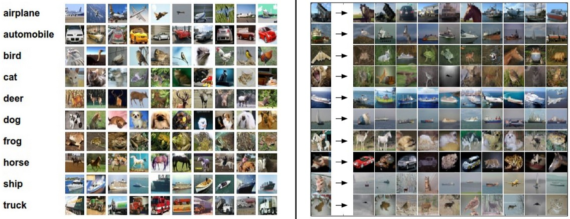
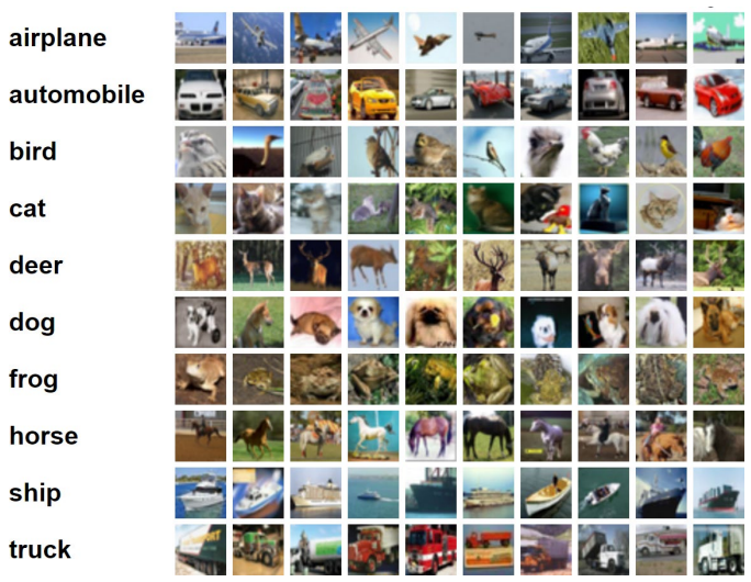
In the context of image classification, a linear classifier is a simple yet fundamental approach. The goal is to map an input image to one of several predefined categories or classes. For example, the CIFAR-10 dataset contains images, each belonging to one of 10 different categories such as “airplane,” “cat,” “dog,” or “truck.” Each image is represented by its pixel values, and the classifier must determine which category the image belongs to.
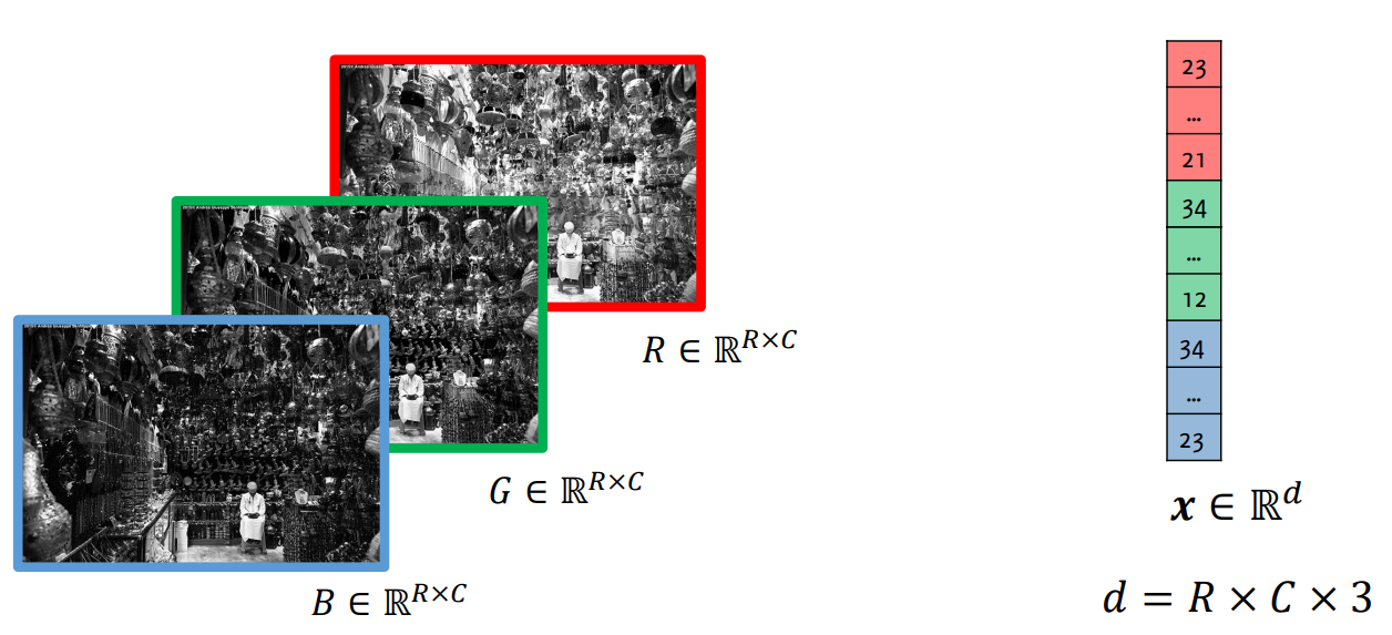
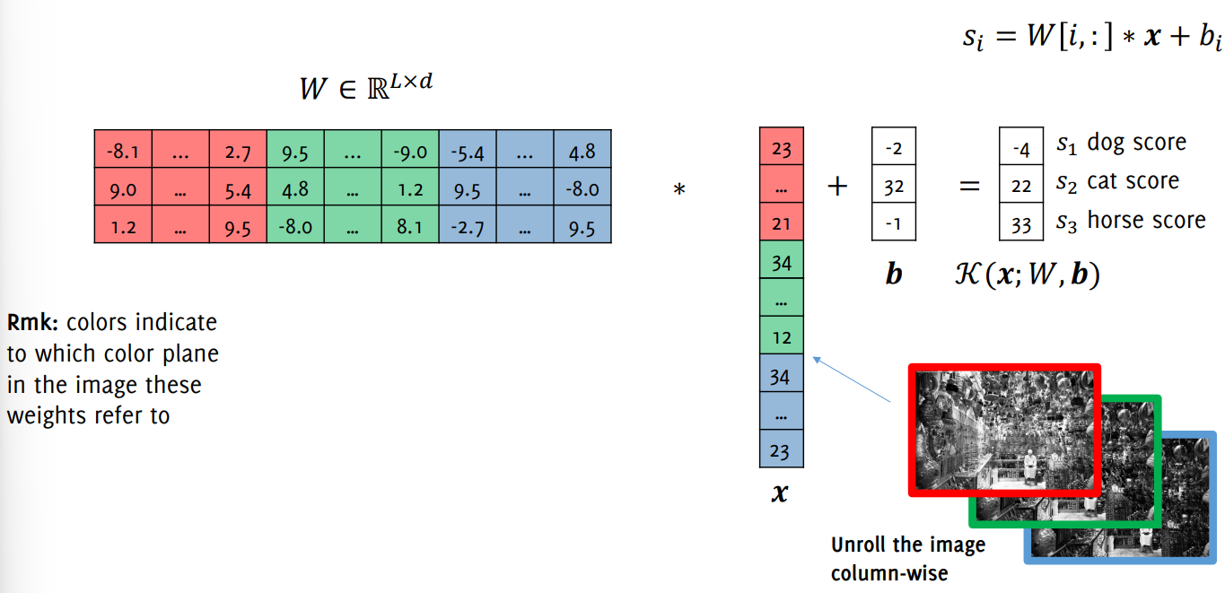
An image, denoted as , must be flattened into a vector , where . Flattening means converting the image’s two-dimensional spatial structure into a one-dimensional vector while preserving the pixel intensities.
Example
For example, in the CIFAR-10 dataset, each image is pixels with 3 color channels. Flattening results in a vector of length . The vector is organized such that the first values represent the red channel, the next values represent the green channel, and the final values represent the blue channel.
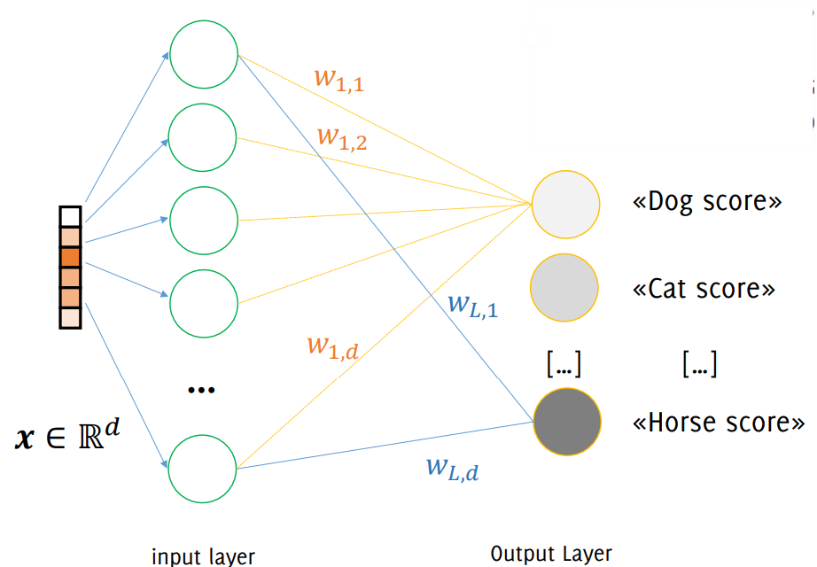
A linear classifier for this problem can be represented by a single-layer neural network. This network has input neurons (one for each pixel value in the flattened image) and output neurons (one for each class). The network computes a score for each class, and the class with the highest score is selected as the predicted label.
The classifier can be defined as a linear function that maps the input vector to an output vector of class scores :
where:
is the weight matrix, with each row corresponding to the weights associated with class .
is the bias vector, which introduces additional flexibility in the classification.
is the flattened input image.
The output of the classifier is a vector of 10 scores, one for each class. The predicted label is the index of the class with the highest score:
Example: CIFAR-10 Classifier
Consider a simple linear classifier for the CIFAR-10 dataset. Each image is flattened into a vector of size 3072, and the classifier predicts one of 10 labels:
For each image, the classifier computes the scores for all 10 categories using the linear function . The label corresponding to the highest score is selected as the predicted class.
The structure of the linear classifier can be visualized using the following summary (generated by model.summary() in a deep learning framework like TensorFlow or PyTorch):
Here, the input layer has 3072 neurons (flattened image), and the output layer has 10 neurons (one for each class). The total number of parameters is calculated as:
This represents the weights connecting the input neurons to the output neurons, plus the bias terms.
When considering the use of a deep neural network with an architecture like the one described (where the number of neurons in each layer progressively decreases), dimensionality and the number of parameters become critical factors. This approach is aimed at reducing the dimensionality of the input while still capturing the most important features for classification.
Network with a Hidden Layer (Half the Input Size)
For the CIFAR-10 dataset, which has input images flattened into vectors of size (since ), a network with an intermediate hidden layer can be constructed as follows:
First Layer (Input): The input layer consists of neurons (one for each pixel value in the flattened image).
Second Layer (Hidden): The hidden layer has neurons, which is half the size of the input layer. This reduction in size forces the network to focus on the most important features of the image.
Output Layer: The output layer has neurons, one for each class in the CIFAR-10 dataset.
Parameter Calculation
First Layer to Hidden Layer: The number of parameters is given by:
This includes the weight matrix , which has parameters, plus the bias terms (one for each neuron in the hidden layer).
Hidden Layer to Output Layer: The number of parameters is given by:
This includes the weight matrix , plus bias terms, one for each class in the output layer.
Thus, the total number of parameters in the network is:
This is a substantial number of parameters for a network that is still relatively simple (only one hidden layer).
Linear Classifier (No Non-Linearity)
In the case of a linear classifier, the network is represented by the following equation:
where:
is the flattened input image.
is the weight vector for class .
is the bias term for class .
The network computes a score for each class based on the weighted sum of the input pixels, and the class with the highest score is selected as the predicted label. The function mapping the input to the output is linear:
where:
is the weight matrix (with for the 10 classes and for the flattened image size).
is the bias vector.
The predicted class is the one with the highest score:
where, the softmax function is not required, because it only normalizes the scores, and it does not change the relative ordering of the scores. As long as we are only interested in the class with the highest score, we can skip the softmax step.
The weights in the network play a crucial role in determining the class of the input image. The values in the weight matrix highlight the most important pixels (or regions) in the image for classification. For example, in a linear classifier, if certain pixel intensities are strongly associated with a particular class (e.g., red pixels for “airplane” or green pixels for “forest”), the corresponding weights for those pixels will have larger magnitudes for that class.
Without non-linear activations between layers, stacking multiple layers in a neural network does not increase the model’s capacity to learn complex patterns. Mathematically, if we stack multiple layers without any non-linearity, the entire operation can be collapsed into a single linear transformation:
This equation shows that even with multiple layers, the operation is equivalent to a single-layer model if there is no non-linearity (like ReLU, sigmoid, or tanh) between the layers. This is why non-linearity is critical in deep learning models—it allows the network to learn more complex and non-linear relationships between the input and the output.
Training the Linear Classifier
In training a linear classifier, the goal is to find the optimal parameters and that minimize the loss function over the training set . The parameters and are found by minimizing the loss function over all training examples in the dataset . The optimization problem is:
where:
represents the th input image, flattened into a vector.
is the corresponding label for the th image.
is the loss function, which measures how well the model is classifying the input .
Loss Function
The loss function evaluates the classifier’s performance on a given training example. A good classifier will assign higher scores to the correct class and lower scores to incorrect classes. The loss function could take different forms:
Hinge Loss (SVM):
where is the score for class , and is the score for the correct class.
Cross-Entropy Loss:
This is often used in conjunction with a softmax function, which normalizes the scores into probabilities.
The loss function should be minimized to achieve better classification performance.
To avoid overfitting and ensure a unique solution with desired properties (e.g., small weights), a regularization term is added. The regularized optimization problem becomes:
where:
is the regularization parameter that controls the trade-off between fitting the training data and regularizing the model.
is a regularization function that penalizes large weights or biases. Common choices for include:
L2 Regularization (Ridge):
L1 Regularization (Lasso):
The regularization helps improve generalization by discouraging overly complex models with large weights.
Training via Gradient Descent
The optimization problem is typically solved using gradient descent or its variants, such as:
Stochastic Gradient Descent (SGD): Updates the parameters based on a single or small batch of training examples at each step.
Momentum: Accelerates SGD by adding a momentum term that helps smooth the updates.
Adam: An adaptive learning rate optimizer that combines the benefits of both SGD and Momentum.
At each iteration, the gradients of the loss function with respect to the weights and biases are computed, and the parameters are updated accordingly:
where is the learning rate, which controls the step size of the updates.
Once the training process converges, the learned parameters and are stored, and the training set can be discarded. The classifier can now be used to predict the labels of new input images based on the learned weights and biases.
The prediction for a new image is made by computing the class with the highest score:
Thus, the model assigns the new image to the class that corresponds to the largest score.
Geometric Interpretation of a Linear Classifier
A linear classifier assigns a score to each class based on a weighted sum of the input features (which can be thought of as pixel intensities in an image). This is done by computing the inner product between a weight vector associated with the class and the input vector representing the image, followed by the addition of a bias term :
This is a linear transformation that evaluates how well the input image matches the learned weights for each class. The classifier computes scores for all classes independently and selects the class with the highest score as the predicted class. The weights and biases and are learned during training.
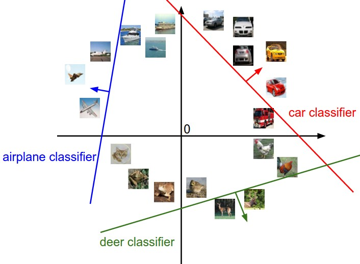
In geometric terms, each weight vector represents a hyperplane in the input space (where is the dimension of the input). In the case of a 2D input (i.e., ), the function would be:
The equation defines a line that separates the space into regions where the score is positive or negative. In higher dimensions, this becomes a hyperplane. The classifier assigns each point (image) to the class with the highest score, and these hyperplanes act as decision boundaries between classes.
In another interpretation, we can view each weight vector as a template that the classifier tries to match against the input image. The classification score for class is computed as a correlation between the input image and the template . The classifier selects the template that best matches the input, which can be seen as finding the highest similarity score.
In Python notation, the inner product computation would be:
s = np.inner(W[i,:], x) + b[i]
where, is the template for class , and the function np.inner() computes the dot product between the template and the image. The bias adjusts the score accordingly.
Example of Template Matching
Consider the CIFAR-10 dataset, which contains images of objects such as birds, frogs, cars, and planes. Each class has a learned template that matches typical features of that class:
Birds and frogs may be associated with green backgrounds, so the weight vectors for these classes might learn to pick up on green pixels.
Planes and boats often have blue backgrounds, leading to templates that emphasize blue pixels.
Cars might typically appear as red, and the weight vector for the car class would focus on red pixels.
The score for each class is then the correlation between the input image and the learned template for that class. For example, the template for class 1 is , and the score can be computed as:
where represents the intensity of pixel in the input image and is the corresponding weight in the template for class 1.
Linear classifiers can be thought of as performing template matching across different classes. The weights act as learned templates that best match the input images for each class. The classification is based on the similarity (inner product) between the image and the templates.
This interpretation is simple and intuitive, but it has limitations. Linear classifiers can only separate data that is linearly separable, meaning the decision boundaries between classes must be straight lines or hyperplanes. When the data is more complex and not linearly separable, more sophisticated models, such as neural networks with nonlinear activations or convolutional neural networks (CNNs), are required to capture the intricate patterns in the data.
Templates Learned on the CIFAR-10 Dataset
The CIFAR-10 dataset consists of a diverse set of images across ten classes. The learned templates for each class reveal interesting insights into how linear classifiers interpret and classify the images:
Horses:
The dataset includes images of horses looking in different directions. As a result, the learned template for horses might reflect this variability, leading to a “two-headed” appearance. This means the classifier is attempting to capture features that can represent horses regardless of their orientation.
Image Invariance:
If you want a model to recognize images that are invariant to transformations, such as left-right flips, it’s essential to train the network on a dataset that includes these variations. This is why techniques like image augmentation are critical during training. By artificially increasing the diversity of the training set (e.g., flipping images, adjusting brightness, etc.), the model learns to generalize better and become robust to such transformations.
Background Colors:
Birds and Frogs: The backgrounds of these classes are typically green. Hence, the learned templates for birds and frogs might focus on features that emphasize green hues in the images.
Planes and Boats: These classes often feature blue backgrounds, which influences their corresponding templates to prioritize blue pixels.
Cars: Cars frequently appear as red in the dataset, so the template for the car class would likely highlight red features.
Limitations and Importance of Linear Classifiers
While linear classifiers offer a straightforward approach to classification and are interpretable, their simplicity can lead to limitations:
Model Complexity: The linear classifier’s inability to capture complex patterns means it may underperform on more intricate datasets. The learned templates can become overly simplistic, leading to suboptimal performance, especially in cases where classes have overlapping features or non-linear boundaries.
Interpretability: One significant advantage of linear classifiers is their interpretability. The weights can be directly understood as the importance of different features (or pixels) in determining the class. In contrast, more complex models, such as deep neural networks, often function as “black boxes,” making it challenging to understand how they arrive at specific predictions.
Is Image Classification a Challenging Problem?
Yes, image classification is a challenging problem due to several factors that arise from the complexity of visual data and the limitations of existing models and approaches. These challenges can be grouped into a few key areas:
Dimensionality
Label ambiguity
Transformations
Intra-class variations
Similarity
Dimensionality
Images are inherently high-dimensional data, and this dimensionality makes classification difficult. Consider the CIFAR-10 dataset, which consists of relatively small RGB images. Even with these small images, each image has pixels:
Compared to traditional datasets used in machine learning (such as those in the UCI Machine Learning Repository, which have relatively few attributes), images are much larger in terms of both features and storage requirements. Many datasets in traditional machine learning have less than 500 attributes, whereas even a small image like those in CIFAR-10 has over 3,000.
The challenge arises not just from the large number of pixels but also from the fact that each pixel is part of a larger structure (i.e., the image), and its value can be influenced by numerous factors (such as lighting, background, and orientation). Moreover, training models like Convolutional Neural Networks (CNNs) requires handling batches of such high-dimensional data and corresponding activations, all of which have to fit into memory.
Label Ambiguity
Another key challenge in image classification is label ambiguity. An image can often be labeled in multiple valid ways depending on the context. For example, a picture of a car could be labeled as “car,” but depending on the setting, it could also be labeled as “vehicle,” “transportation,” or even “street scene.” This ambiguity makes it difficult to define the exact label for many images, which in turn complicates model training.
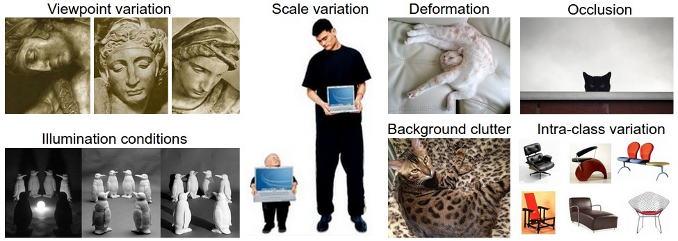
Transformations
Real-world images often undergo transformations that dramatically alter their appearance while keeping the label intact. Some common transformations include:
Illumination changes: Lighting variations can change pixel values significantly.
Deformations: Non-rigid objects (e.g., animals, people) can take on different shapes.
Viewpoint changes: Objects can be viewed from different angles.
Occlusion: Parts of an object might be hidden.
Background clutter: Objects might appear in front of complex or noisy backgrounds.
Scale variation: Objects might appear larger or smaller depending on their distance from the camera.
Models need to be invariant to such transformations to achieve high performance, and this is often difficult to ensure without using extensive augmentation techniques during training.
Intra-Class Variation
There can be significant variation within the same class, especially in large datasets. For example, in the CIFAR-10 dataset, images of cars can include sports cars, sedans, trucks, etc., each looking very different from one another. Similarly, animals like dogs can vary dramatically in breed, color, and posture.
This intra-class variation introduces the need for models to learn a more generalized representation of each class, capturing the essence of the object or scene, rather than overfitting to specific examples.
Perceptual Similarity vs. Pixel Similarity
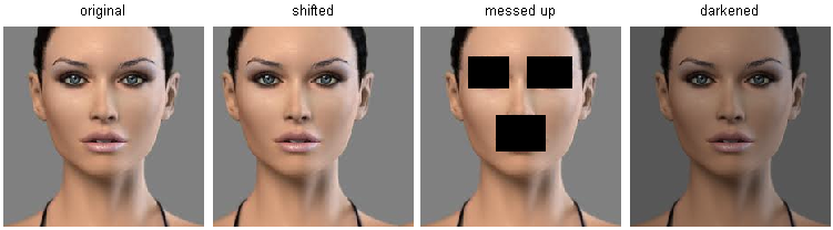
One of the fundamental difficulties in image classification lies in the fact that perceptual similarity between images does not correspond to pixel-wise similarity. Two images may appear very similar to a human observer (e.g., a dog sitting in different poses), but their pixel-wise differences could be large due to changes in lighting, background, or small shifts in the object’s position.
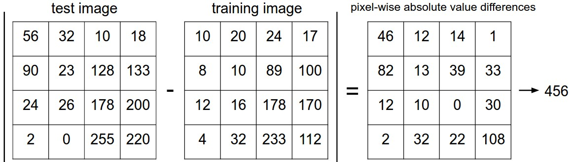
A common baseline approach is to classify an image based on the label of the closest image in the training set, using distance metrics such as Euclidean distance or Manhattan distance:
With distances typically defined as:
Euclidean Distance:
Manhattan Distance:
While distance-based methods are simple, they are often ineffective because pixel-wise similarity does not correspond to how humans perceive similarity. For instance, shifting an object slightly in an image could result in a large pixel-wise distance but would not alter the perceived object.
K-Nearest Neighbors (KNN) Classifier
In the K-Nearest Neighbors (KNN) approach, the classification of a test image is determined by the labels of the closest images from the training set. Specifically, the prediction is made by assigning the most frequent label among these closest neighbors:
where is the set of nearest training images to the test image , and the distance between images is typically calculated using a distance metric like Euclidean or Manhattan distance.
(number of neighbors): The value of can significantly affect the classifier’s performance. Small values might lead to overfitting, while larger values may smooth over variations but could miss finer details.
Distance metric: The distance measure (Euclidean, Manhattan, etc.) used to compare images plays a crucial role in how the classifier behaves. However, finding an appropriate metric for high-dimensional data like images is not straightforward.
Pros
Cons
Easy to understand and implement
Computationally expensive at test time, especially when the training set () is large and the feature dimension () is high.
No training time required: The algorithm directly operates on the data without building a complex model.
Memory intensive: The entire training set must be stored, which can be problematic with large datasets.
Distance interpretation: Pixel-wise distance measures may not correspond to perceptual similarity, especially for high-dimensional data like images.
A key challenge with KNN is that pixel-wise distance, such as Euclidean or Manhattan distance, does not capture perceptual similarity between images. For example, in the case of images, slight variations like shifts, lighting changes, or different orientations can result in large pixel-wise differences even though the images represent the same object.
Consider three different images that have the same pixel-wise distance from an original image:
While these images have similar pixel-wise distances, they can look perceptually very different. This issue makes it difficult for KNN to be effective on image classification tasks, especially in datasets like CIFAR-10, where images differ in subtle but perceptually meaningful ways.
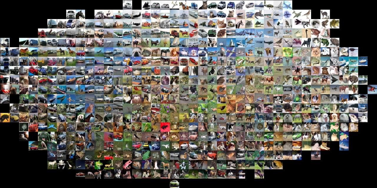
Applying KNN with a pixel-wise distance metric (such as Euclidean distance) on CIFAR-10 results in poor performance because the distance metric does not effectively capture the perceptual differences between images. Even though the pixel-wise distances may be similar, the images may belong to different classes, making KNN unreliable.