B - Review of Probability Theory

---

In the domain of Artificial Intelligence (AI), an agent rarely possesses complete or absolute knowledge regarding its operating environment. This inherent limitation necessitates that AI systems manage and reason under uncertainty. This uncertainty stems fundamentally from issues such as:

• partial observability, where the agent’s sensors do not capture the entire state space;
• noise in sensor data, which introduces inaccuracies into observations;
• the sheer immense complexity of modeling real-world phenomena. To formalize and quantify this lack of certainty, probability theory is employed, providing the essential mathematical framework for coherent reasoning with incomplete information.

Fundamental Principles of Probability

The foundation of probability theory rests on the notion of a possible world or outcome, denoted by . Every conceivable state of the environment, resulting from an action or an observation, belongs to the sample space, . This sample space is defined as the exhaustive and mutually exclusive set of all possible outcomes.

The Axioms of Probability

The likelihood of any specific possible world being the actual state of reality is quantified by its probability, . These probabilities must rigorously adhere to the following two axioms of probability, which ensure a consistent measure:

1. Axiom of Bounds (Non-negativity and Normalization): The probability assigned to any single possible world must be a real number inclusively bounded between zero and one.

   This axiom establishes that probabilities are non-negative and can never exceed certainty.

2. Axiom of Total Probability (Exhaustiveness): The summation of the probabilities for all distinct possible worlds that constitute the sample space must precisely equal one.

   This ensures that one of the possible outcomes must occur.

Case Study: Illustrating Probability with Dice Rolls

The mechanism of rolling dice provides a clear and tangible visualization of these core probabilistic concepts.

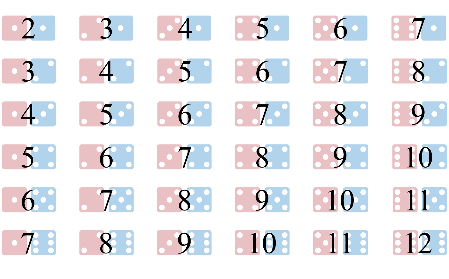
When considering a single, standard, fair die, the sample space consists of six distinct, equally likely outcomes: . By the total probability axiom, the probability of any specific side being rolled is .

The scenario is scaled up by rolling two distinguished dice (e.g., a Blue die and a Red die). The combined sample space significantly increases; there are distinct and equally probable outcomes, such as (Blue=1, Red=1) or (Blue=6, Red=3). The probability of any one specific outcome, , is consequently .

We are often concerned not with atomic outcomes, but with an event, which is formally defined as a subset of the sample space. The probability of an event is calculated by summing the probabilities of all the atomic outcomes that satisfy the event’s condition.

• Example A (Event: Sum = 12): This event is satisfied by only one outcome: (Red=6, Blue=6). Therefore, the probability is: .

• Example B (Event: Sum = 7): This event is satisfied by six outcomes: . The probability is thus calculated as the sum of these six atomic probabilities: .

This demonstration formally explains why a sum of seven is the most probable result, or modal outcome, in two-dice games, while sums of two and twelve are the least probable.

Types of Probabilistic Quantifications

Probability theory distinguishes between different measures of belief based on the information available to the agent.

Unconditional (Marginal or Prior) Probability

Unconditional probability, also frequently termed marginal probability or prior probability, represents the agent’s degree of belief in a specific proposition, , in the absolute absence of any contextual evidence. It is derived by considering the entire sample space or dataset as a whole without any conditional filtering. Its definition is simply .

A classic example is calculating the general probability of rain based solely on historical climatic averages, before any current weather observations are made. In the dice scenario, is an unconditional probability.

Conditional (Posterior) Probability

Conditional probability, or posterior probability, represents a revised degree of belief in a proposition, , after some specific evidence (or condition), , has been observed. This process is essentially an update of the sample space. The new reference space, or effective sample space, becomes the set of outcomes consistent only with the observed evidence , rather than the entire original space . This is denoted as , read as “the probability of given .” For instance, an agent might ask, “What is the probability of rain, given that the sky is heavily cloudy?”

Example

To grasp this concept, consider calculating the probability of the sum being 12 () given the evidence that the Red Die is showing a 6 ().

1. Prior State: Initially, is .
2. Evidence Conditioning: The evidence restricts the effective sample space to only the six outcomes where the Red Die is 6:

All other 30 outcomes are irrelevant under this condition.

3. Posterior Calculation: Within this restricted, new sample space of size 6, only one outcome, (Red=6, Blue=6), results in a sum of 12. Therefore, the conditional probability is:

   The knowledge that the Red Die is 6 has significantly increased the probability of the sum being 12, demonstrating the mechanism of belief updating.

The Mathematical Definition and Product Rule

The relationship between conditional, unconditional, and joint probability is formalized by the mathematical definition of conditional probability:

Definition

the conditional probability of given is the probability of both events occurring simultaneously (joint probability, ), normalized by the unconditional probability of the evidence .

This equation holds under the condition that . The notation represents the Joint Probability, signifying that both and are true in the resulting world state.

Rearranging this fundamental relation yields the crucial Product Rule (or Chain Rule for two variables), which allows for the calculation of the joint probability of two events through their conditional and marginal probabilities:

Alternatively, due to the commutativity of the conjunction operator , the rule can also be stated as:

This rule is foundational, enabling the calculation of the probability of complex events by decomposing them into a sequence of simpler, conditional probabilities.

Random Variables and Probability Distributions

The concept of a random variable is essential in bridging the abstract notion of a sample space of outcomes () with numerical or categorical representations that are more amenable to mathematical analysis and computation within AI systems.

The Concept of Random Variables

A random variable (RV), conventionally denoted by an uppercase letter (e.g., ), is formally defined as a function that maps every outcome in the sample space () to a specific, measurable value, typically a real number or a categorical label. This transformation allows probability theory to operate on structured domains of values rather than on arbitrary outcomes. The domain of a random variable is the set of all possible values it can assume.

For instance, in the context of the dice case study, the raw outcome is a pair like (Red=2, Blue=5). A random variable representing the sum of the dice maps this outcome to the value 7. The domain of the variable is .

Examples of Random Variables and their domains include:

• Discrete Variable : Represents the outcome of a single die toss, with the finite and countable domain of .
• Categorical Variable : Represents the environmental state, with a non-numeric, discrete domain such as .
• Categorical Variable : Represents an airline status, with the domain .

Probability Distributions

A probability distribution is the complete specification of the probability for every single value within a random variable’s domain. It provides a comprehensive model of the uncertainty associated with that variable. For a discrete random variable with domain , the distribution assigns a probability for every value . Critically, in accordance with the Axiom of Total Probability, the sum of all assigned probabilities must normalize to unity: .

Example

Consider the example of the categorical random variable status at an airport. Its probability distribution, derived from historical data, might be:

This distribution, often represented compactly using vector notation as , completely characterizes the state of belief regarding the variable. This complete probabilistic description is essential for AI agents, as it allows them to calculate expected utilities and make optimal decisions, such as determining the best time to arrive at the airport given the probability of a delay. This is a crucial foundation for subsequent concepts like joint and conditional probability distributions that involve multiple variables.

Independence in Probability Theory

The concept of independence is one of the most powerful and computationally advantageous assumptions in probability theory and is critically leveraged across various Artificial Intelligence (AI) algorithms, such as the highly practical Naive Bayes classifier. It allows for significant simplification of the joint probability space, making complex problems tractable.

Definition

Two events, and , are formally defined as probabilistically independent if the knowledge or occurrence of one event imparts no change to the likelihood of the other event occurring.

In the context of rational belief updating, this signifies that observing the evidence does not alter our prior degree of belief in .

This relationship is expressed mathematically using conditional probability:

This reads as: the probability of given is identical to the unconditional (marginal) probability of . Symmetrically, the independence relationship is mutual: if is independent of , then is necessarily independent of , meaning .

The fundamental power of independence is realized through the simplification of the general rule for calculating joint probability.

The General Product Rule (or the Law of Total Probability for joint events), which applies universally to any two events, is:

When and are established as independent, the conditional term is replaced by the marginal probability , leading to the Simplified Product Rule for Independent Events:

This simplified formula is frequently employed as the definitive test for independence: if the observed joint probability of two events equals the product of their individual marginal probabilities, the events must be independent. This factorization is what provides computational efficiency, particularly in machine learning models where high-dimensional joint distributions are otherwise difficult to calculate.

Case Study: Differentiating Independence and Dependence

To solidify the distinction, it is beneficial to analyze two separate scenarios involving dice.

Scenario A: True Independence (Separate Trials)

Consider the outcomes of two distinct, physically separated dice: a Red Die and a Blue Die. We are interested in the joint event that the Red Die shows a 6 () and the Blue Die shows a 6 ().

• Rationale: The physical realization of the Red Die’s face is causally disconnected from that of the Blue Die. Therefore, knowing provides zero information about .

• Calculation using Independence: Since the events are independent, we apply the simplified product rule:

• Conclusion: The joint probability calculated via the independence assumption, , accurately reflects the probability of that specific outcome in the total sample space of 36 possibilities, confirming that the events are independent.

Scenario B: Dependence and Mutual Exclusivity (Single Trial)

Now consider two outcomes on the same single Red Die: Rolling a 6 () and Rolling a 4 ().

• Test for Independence (Hypothetical): If the two events were hypothetically independent, their joint probability would be the product of their marginals:

• Reality (Actual Joint Probability): It is physically impossible for a single, fair die to simultaneously land on two different faces. The actual joint probability of this occurrence is zero:

• Conclusion: Since the actual joint probability () does not equal the probability required for independence (), the events are definitively not independent; they are dependent.

The source of this dependence is that the events are mutually exclusive (or disjoint). Mutual exclusivity is a strong form of dependence. If we know that the outcome is 6, the conditional probability of the outcome also being 4 drops from its prior value of down to . Because the observation of one event critically alters the belief in the other, dependence is clearly established.

This is formally confirmed by applying the General Product Rule:

Bayes’ Rule: The Foundation of Probabilistic Inference

Bayes’ Rule, named after the Reverend Thomas Bayes, is the cornerstone of probabilistic inference within Artificial Intelligence. It provides a formal, mathematical mechanism for updating an agent’s beliefs (i.e., probabilities) in a hypothesis when new, relevant evidence is observed. Crucially, Bayes’ Rule facilitates the inversion of conditional probabilities, enabling the calculation of when the typically more accessible causal probability is known.

Proof

The rule is derived directly from the fundamental symmetry inherent in the Product Rule for joint probabilities. As established, the joint probability of two events, and , must be independent of the order of calculation:

1. Joint probability of and expressed through the conditioning on :
2. Joint probability of and expressed through the conditioning on :

By equating these two expressions for the same quantity, , we establish the equality:

Dividing both sides of this equation by the marginal probability yields the standard formulation of Bayes’ Rule:

In the context of machine learning and AI, the components of Bayes’ Rule map directly to the process of hypothesis testing and belief updating:

• (Posterior Probability): This is the ultimate goal of the calculation. It represents the updated belief in the hypothesis after observing the evidence .
• (Likelihood): This term represents the probability of observing the evidence assuming the hypothesis is actually true. This is often an estimate of the causal relationship and is typically easier to ascertain from empirical data (e.g., “What is the likelihood of a specific symptom given a known disease?”).
• (Prior Probability): This represents the initial degree of belief in the hypothesis before any evidence is taken into account. It is the unconditional or marginal probability of the hypothesis.
• (Marginal Evidence): This is the normalizing constant, representing the overall, marginal probability of observing the evidence under all possible circumstances (hypotheses).

Example: Predictive Weather Inference

The power of Bayes’ Rule is illustrated by transitioning from causal observation to diagnostic inference, such as predicting rain based on cloud observation.

The Inference Problem: Determine , the probability of rain given a cloudy morning.

Known Empirical Data:

1. Likelihood (): An 80% chance of a cloudy morning when the afternoon is rainy.

2. Prior (): A 10% base rate for rainy afternoons.

3. Evidence (): A 40% base rate for cloudy mornings overall.

Bayesian Calculation:

Substituting these values into the rule to compute the posterior probability:

Despite the strong likelihood that cloudy mornings lead to rain (0.8), the posterior probability of rain given a cloud is only 20%. This seemingly counter-intuitive result is mathematically sound and underscores the importance of the prior probability () and the commonality of the evidence (). Since most cloudy mornings (60%) do not result in rain, the high base rate of clouds dilutes the diagnostic power of the evidence.

Bayes’ Rule is instrumental because it effectively reverses the direction of probabilistic inference, transitioning from the typically available causal knowledge to the required diagnostic knowledge.

• Causal Direction (): Data is often collected in the causal direction.

,

This describes the mechanism or system performance (e.g., test sensitivity).

• Diagnostic Direction (): This is the direction needed for practical decision-making and real-world inference.

, This answers the critical question: "Given the observed effect (evidence), what is the most probable underlying cause (hypothesis)?"

In clinical diagnosis, for example, a test may have high sensitivity (high ), but a low prior probability of the disease coupled with the test’s specificity can result in a surprisingly low posterior probability . Bayes’ Rule is the only correct way to integrate the likelihood, the prior, and the evidence to provide an accurate diagnostic assessment.

Joint Probability Distributions

While an individual random variable provides insight into an isolated phenomenon, the true complexity of real-world environments addressed by Artificial Intelligence necessitates understanding the interdependencies and interactions among multiple variables. This comprehensive view is captured by Joint Probability Distributions.

A joint probability distribution (JPD) specifies the probability for every single possible assignment of values to a set of two or more random variables, thus providing a complete probabilistic model of that subset of the world. For a set of random variables , the JPD is denoted as , and its full representation is often referred to as the Full Joint Probability Distribution if it covers all relevant variables in the domain.

The JPD is the ultimate source of knowledge, as any probabilistic query concerning these variables can be derived directly from it. Critically, as with any probability distribution, the sum of probabilities across all combinations of variable assignments in the JPD must satisfy the normalization axiom and equal .

Example: Weather Patterns Joint Table

Consider the two Boolean random variables:

• : (True or False)
• : (True or False)

The joint distribution is represented as a table that lists the probability of each unique combination of outcomes, which are the atomic worlds in this restricted sample space:

(Morning)	(Afternoon)	Joint Probability
True	True	0.08
True	False	0.32
False	True	0.02
False	False	0.58

The value means that the specific state where it is cloudy in the morning and it rains in the afternoon occurs of the time. The table provides a holistic picture, showing that non-cloudy, non-rainy days (False, False) are the most probable single state at .

Probability Rules and Manipulation

The JPD is powerful because it allows us to calculate any other probability, whether marginal or conditional, through three foundational rules of probability manipulation: Negation, Inclusion-Exclusion, and Marginalization.

Negation

The Negation Rule provides a simple method for determining the probability of an event’s complement. Since an event and its negation (not ) are mutually exclusive and collectively exhaustive, their probabilities must sum to one:

Inclusion-Exclusion Principle

When calculating the probability of the disjunction of two non-mutually exclusive events—the probability that event or event occurs, denoted —a simple summation of their marginal probabilities would erroneously double-count the probability of the joint event where both occur. The Principle of Inclusion-Exclusion corrects this by subtracting the joint probability:

This ensures that the outcomes where both and are true are counted exactly once.

Marginalization (Summing Out)

Marginalization, often referred to as “summing out,” is the mechanism used to extract the probability of a subset of variables from a larger joint distribution by aggregating (summing) the probabilities over the possible values of the variables we wish to ignore or remove from consideration. The resulting distribution is the marginal probability distribution for the remaining variables.

For two Boolean variables, and , the marginal probability of is found by summing the joint probabilities of across all possible states of :

For a more generalized case where variable has a domain of values , the marginal probability of is given by:

This formula represents the fact that can occur with any possible value of .

Example Application: Recovering Marginal Probability

Using the Joint Weather Table, we can recover the marginal probability of a Cloudy Morning (). We sum the probabilities for all outcomes where :

This calculation confirms the marginal probability of , demonstrating that the full joint distribution contains all the information required to determine any marginal or conditional probability.

Conditioning: The Law of Total Probability

The technique of Conditioning is an indispensable method for calculating marginal probabilities without requiring the full joint distribution, provided a set of conditional and prior probabilities are known. It effectively combines the Marginalization Rule with the Product Rule, resulting in the Law of Total Probability. This law is crucial for systems that must compute the overall likelihood of an event by aggregating probabilities across a mutually exclusive and exhaustive set of intermediate states or hypotheses.

The Law of Total Probability Formula

The Law of Total Probability states that the probability of an event can be calculated by summing the joint probabilities of and every possible state of a related variable . By substituting the Product Rule, , into the marginalization formula, we obtain the expression for conditioning.

If the variable is Boolean (taking on values or ):

If the conditioning variable has a discrete domain of mutually exclusive and exhaustive values , the marginal probability of is calculated by summing over all possible states of :

The set of events forms a partition of the sample space, ensuring that every possible outcome is accounted for exactly once.

Interpretation as a Weighted Average

The conditioning formula has a powerful interpretation as a weighted average. It asserts that the unconditional (marginal) probability of the event is the average of the conditional probabilities of given each state of the conditioning variable , where each conditional term is weighted by the prior probability of that conditioning state occurring.

This methodology provides a structured approach for an intelligent agent to reason about the overall likelihood of a complex event by decomposing the problem into simpler, discrete cases based on the values of .

For example, an AI agent might want to compute the overall probability of a flight being delayed ( ) by conditioning on the possible weather conditions (). The probability of delay is averaged across all weather states (sunny, cloudy, stormy), weighted by how often each weather state actually occurs.

This is a fundamental technique used in probabilistic modeling to manage complexity and calculate marginal probabilities without exhaustively enumerating the full joint space.