Branch prediction is a crucial technique used in modern processors to mitigate the impact of branch hazards, which arise when the outcome of a conditional branch instruction is unknown at the time of fetching subsequent instructions. Instead of stalling execution until the branch decision is resolved, branch prediction speculatively assumes an outcome—either the branch will be taken or not taken—and proceeds under that assumption.
If the prediction is correct, the processor continues execution seamlessly
If the prediction is incorrect, the speculative instructions must be discarded, leading to performance penalties.
To address the performance loss due to branch hazards, two broad categories of branch prediction techniques are employed:
Static Branch Prediction Techniques: These techniques determine the branch outcome at compile time, meaning the predicted behavior of a branch remains fixed throughout program execution.
Dynamic Branch Prediction Techniques: These methods allow the branch predictor to adapt at runtime by monitoring past branch behavior and updating predictions accordingly.
A combination of these two approaches is often used to optimize performance. Regardless of the prediction technique employed, one fundamental requirement remains: the processor state and registers must remain unchanged until the actual branch outcome is definitively known to ensure the correctness of execution.
Static Branch Prediction Techniques
Definition
Static branch prediction is a method in which the expected outcome of a branch instruction is determined at compile time.
This approach is particularly effective for applications in which branch behavior is highly predictable and does not vary significantly across different executions.
Several static branch prediction techniques have been developed, each with varying levels of effectiveness depending on the program’s branch behavior:
Branch Always Not Taken (Predicted-Not-Taken)
Branch Always Taken (Predicted-Taken)
Backward Taken Forward Not Taken (BTFNT)
Profile-Driven Prediction
Delayed Branch
In this analysis, we consider an RISC-V processor optimized for early evaluation of the branch outcome, computation of the branch target address, and update of the Program Counter (PC) in the Instruction Decode (ID) stage.
Summary of Static Branch Prediction Techniques
Technique
Description
Advantages
Disadvantages
Branch Always Not Taken
Assumes branches are not taken, continues sequential execution.
Simple, computationally efficient.
Suboptimal for programs with frequent branch-taken behavior.
Branch Always Taken
Assumes branches are taken, continues at the branch target address.
Effective for loop-intensive code.
Requires early determination of branch target address, suboptimal for forward branches.
Backward Taken Forward Not Taken
Predicts backward branches as taken and forward branches as not taken.
Reduces mispredictions by leveraging common control flow patterns.
Less effective if branch behavior does not follow typical patterns.
Profile-Driven Prediction
Uses empirical data from profiling runs to predict branch behavior.
Higher accuracy, compiler-assisted optimization.
Dependent on the representativeness of training data, potential code size increase.
Delayed Branch
Executes a predetermined number of instructions after a branch before altering control flow.
Reduces performance penalties from branch hazards, effective use of pipeline cycles.
The always not taken branch prediction strategy is one of the simplest and most fundamental approaches. It operates under the assumption that branches will not be taken, meaning execution continues along the sequential instruction flow as if the branch condition were never met.
This technique is particularly effective in scenarios where conditional branches typically evaluate to false, such as IF-THEN-ELSE statements in which the THEN clause is executed infrequently. Since this prediction strategy does not introduce additional complexity in fetching instructions, it is computationally efficient but can be suboptimal for programs with frequent branch-taken behavior.
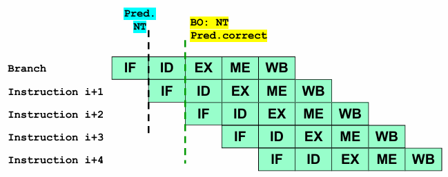
When implementing the Predicted-Not-Taken strategy in a pipeline, the following scenarios arise based on whether the branch is ultimately taken or not:
Correct Prediction (Branch Not Taken):
If the actual branch outcome at the end of the ID stage is not taken, then the prediction is correct.
The processor continues executing the sequential instruction flow without any disruption, maintaining high performance.
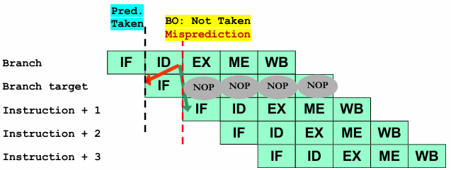
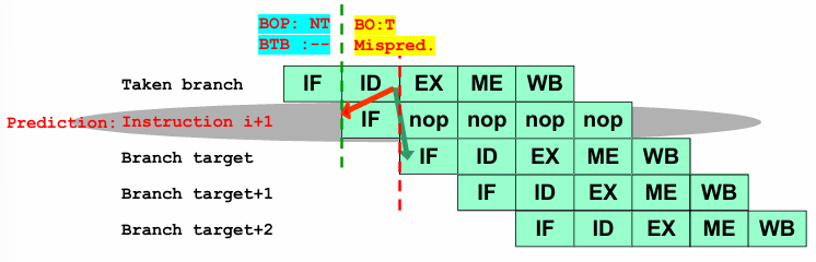
Incorrect Prediction (Branch Taken - Misprediction):
If the actual branch outcome at the end of the ID stage is taken, the prediction was incorrect.
The processor must flush the incorrectly fetched instructions (converting them into NOPs) and fetch the correct instruction from the Branch Target Address.
This results in a one-cycle performance penalty due to the need to discard and reload instructions.
Despite its simplicity, the Predicted-Not-Taken approach is effective in cases where most branches are not taken, as it avoids unnecessary stalls. However, in scenarios where branches are frequently taken, mispredictions become more common, leading to performance degradation due to the repeated need for pipeline flushing.
Branch Always Taken (Predicted-Taken)
The always taken branch prediction strategy is the complementary approach to the always not taken technique. In this method, the processor assumes that every branch instruction will be taken, meaning execution will continue at the Branch Target Address (BTA) rather than sequentially. This prediction technique is particularly well-suited for backward branches, such as those found in DO-WHILE loops, where the loop condition is frequently met, causing repeated iterations.
One challenge with the Predicted-Taken approach is that the processor must determine the Branch Target Address (BTA) as early as possible to avoid unnecessary stalls. Since the BTA is not always immediately available during the Instruction Fetch (IF) stage, a Branch Target Buffer (BTB)—a specialized cache—can be introduced to store previously encountered target addresses. The BTB allows the processor to fetch the correct instruction immediately upon encountering a predicted-taken branch, thereby improving performance.
Assuming that the processor predicts the branch as taken at the end of the IF stage, two possible outcomes exist based on the actual branch decision at the end of the ID stage:
Correct Prediction (Branch Taken):
If the branch is actually taken, the processor has correctly predicted the control flow.
Execution proceeds without interruption, preserving performance.
Incorrect Prediction (Branch Not Taken - Misprediction):
If the branch is not taken, the processor must flush the incorrectly fetched instructions from the BTA (turning them into NOPs) and fetch the correct sequential instruction.
This introduces a one-cycle performance penalty, as the processor must recover from the misprediction.
While the always taken strategy is effective for loop-intensive code, it is suboptimal for forward branches, such as those used in conditional statements where the branch is often not taken. To address this, more refined static prediction strategies have been developed.
Backward Taken Forward Not Taken (BTFNT)
The Backward Taken Forward Not Taken (BTFNT) prediction technique refines the always taken and always not taken strategies by distinguishing between different types of branches based on their direction in the instruction flow:
Backward branches (e.g., loop-ending conditions in DO-WHILE loops) are predicted as taken, assuming the loop will continue iterating.
Forward branches (e.g., conditional statements such as IF-THEN-ELSE) are predicted as not taken, assuming that the most frequent execution path avoids branching.
This approach leverages the common structure of control flow in programs, where loops tend to iterate multiple times, while conditional branches frequently fall through without execution. By tailoring the prediction to these patterns, BTFNT reduces mispredictions compared to simpler static strategies.
Profile-Driven Prediction
Profile-driven prediction is a more sophisticated static branch prediction technique that relies on empirical data rather than fixed assumptions. Instead of applying a universal rule for branch behavior, this method analyzes real execution traces of the program using profiling runs.
Training Phase: The program is executed multiple times with representative input data sets, and the behavior of each branch is recorded.
Prediction Extraction: The gathered data is analyzed to determine how frequently each branch is taken or not taken.
Encoding Prediction Hints: The compiled code is then modified to embed branch hints based on the profiling results, either through compiler annotations or additional instruction bits.
Example
For example, consider a branch with the following execution history:
T T T T NT NT NT NT     --> prediction: NT
T T T T T T T T T NT    --> prediction: T
In the first case, since the branch outcome has shown a strong tendency towards “not taken”, the predictor encodes it as not taken. In the second case, since the branch is predominantly taken, it is predicted as taken.
Advantages
Limitations
Higher Accuracy: Profile-driven prediction provides better accuracy than general static methods because it adapts to the actual behavior of the target program.
Dependency on Training Data: The effectiveness of this method depends on whether the profiling input accurately represents real-world execution patterns. If the training dataset does not generalize well, the predictions may be suboptimal.
Compiler-Assisted Optimization: The profiling phase can be implemented by the compiler or hardware, ensuring minimal overhead at runtime.
Despite its reliance on profiling data, this technique is widely used in compiler optimizations, particularly for programs with stable execution patterns that do not change significantly across runs.
Delayed Branch Technique
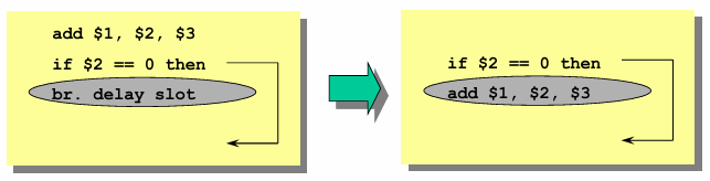
The delayed branch technique is an optimization strategy used to mitigate the performance penalties caused by branch hazards in pipelined processors. Instead of immediately altering the control flow upon encountering a branch instruction, the processor continues executing a predetermined number of instructions after the branch, regardless of whether the branch is ultimately taken or not.
This method requires static scheduling by the compiler, which strategically inserts independent instructions into what is known as the branch delay slot. The delay slot is a pipeline stage where an instruction is executed before the branch takes effect, effectively reducing the number of wasted cycles due to control hazards.
For processors with a single-cycle branch delay (such as MIPS), the compiler must locate one independent instruction to be placed in the delay slot. However, for deeply pipelined architectures, where the branch delay might be multiple cycles, the compiler must identify several independent instructions to fill the slots efficiently.
The primary goal of the compiler is to find a valid and useful instruction to place in the branch delay slot, ensuring that it executes without introducing errors.
The effectiveness of the delayed branch technique depends on the ability of the compiler to:
Identify suitable independent instructions to fill the delay slot.
Minimize performance overhead by avoiding unnecessary instruction duplication.
Ensure correctness by selecting instructions that do not introduce unintended side effects when the branch outcome changes.
For architectures that implement longer branch delay slots (e.g., multiple pipeline cycles), hardware-based dynamic scheduling or speculative execution can be used alongside compiler optimizations to improve performance further. However, in modern architectures, dynamic branch prediction and speculative execution have largely replaced static delayed branch techniques, as they offer more flexibility and higher performance gains.
Scheduling from Before the Branch
In this approach, the delay slot is filled with an independent instruction from before the branch. This instruction is always executed, regardless of whether the branch is taken or not. Since it is never flushed, the compiler must guarantee that its execution does not affect program correctness in either control path.
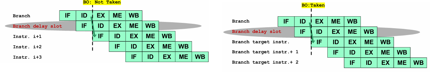
If the branch is not taken, execution continues sequentially, with the delay slot instruction executing normally.
If the branch is taken, the program control jumps to the branch target after executing the delay slot instruction.
This approach is commonly used because it does not require duplicating instructions and ensures efficient use of available pipeline cycles. However, finding a suitable independent instruction can be challenging, especially for complex programs.
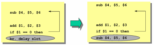
Scheduling from the Branch Target (Taken Path)
In this technique, the instruction placed in the delay slot is taken from the target of the branch (the destination of a taken branch). This strategy is particularly effective for backward branches, such as those found in DO-WHILE loops, where branches are taken with high probability.
The drawback of this approach is that the same instruction must be duplicated if the branch target can be reached via multiple paths. This can lead to code size inflation and may introduce redundancy if not carefully optimized.
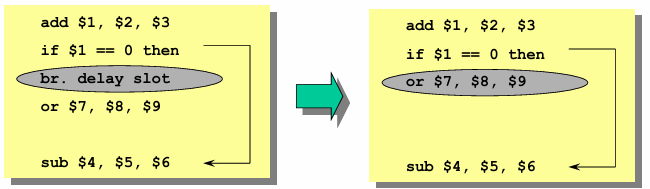
Scheduling from the Fall-Through Path (Not Taken Path)
Here, the delay slot is filled with an instruction from the fall-through path, assuming the branch is not taken. This method is particularly beneficial when forward branches—such as those in IF-THEN-ELSE conditions—are more likely not to be taken. However, if the branch is mispredicted (i.e., the branch is taken instead of not taken), the instruction in the delay slot must either be flushed or be safe to execute even in the taken path.
To ensure correctness, the instruction in the delay slot should meet one of these conditions:
It should be harmless if executed, meaning its execution does not affect the correctness of the program (e.g., writing to a temporary register).
It should be explicitly flushed if the branch outcome contradicts the expected path.
Dynamic Branch Prediction Techniques
Dynamic branch prediction is a hardware-based technique used to anticipate the outcome of branch instructions at runtime, based on their past behavior.
The fundamental goal of this approach is to enhance instruction flow in modern pipelined processors by minimizing the delays caused by branch instructions.
Unlike static prediction methods, where branch outcomes are determined using fixed strategies, dynamic branch prediction adapts to the runtime behavior of branches, updating predictions when necessary to improve accuracy.
At the core of dynamic branch prediction are two key hardware components, both integrated into the instruction fetch (IF) stage of the pipeline.
The Branch Outcome Predictor (BOP)—also known as the Branch Prediction Buffer—is responsible for predicting whether a given branch will be taken or not taken.
The Branch Target Predictor, also referred to as the Branch Target Buffer (BTB), predicts the target address of a taken branch, allowing the processor to fetch the correct instruction immediately.
These two components work together to optimize instruction fetching by reducing the number of stalls caused by control hazards.
The effectiveness of branch prediction depends on how accurately the hardware predicts branch outcomes. There are two primary scenarios in dynamic branch prediction:
Prediction of a Not-Taken Branch:
If the BOP predicts that a branch will not be taken, the processor increments the program counter (PC) to fetch the next sequential instruction. In this scenario, the BTB is not required since there is no need to compute a target address. If the actual branch outcome at the end of the instruction decode (ID) stage confirms that the branch is indeed not taken, the prediction is considered correct, and the processor continues execution without any penalty.
However, if the actual outcome reveals that the branch was taken, the processor must correct the misprediction by flushing the incorrectly fetched instruction, converting it into a NOP instruction, and restarting execution from the correct branch target address. This correction introduces a one-cycle penalty due to the need to refetch the correct instruction.
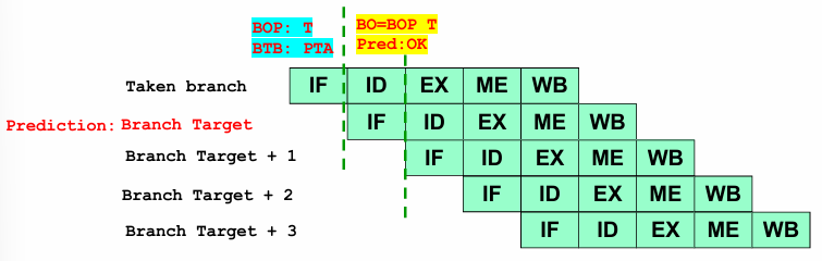
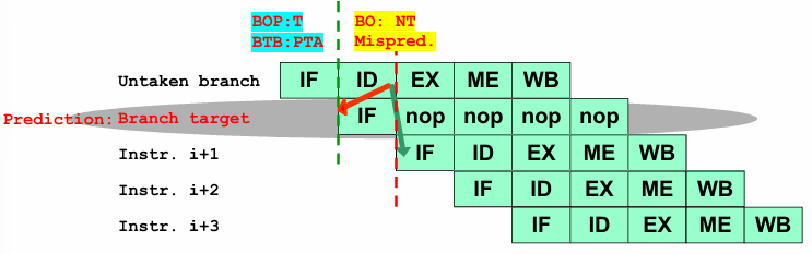
Prediction of a Taken Branch:
When the BOP predicts that a branch will be taken, the BTB supplies the Predicted Target Address (PTA), allowing the processor to prefetch the corresponding instruction. If the branch outcome at the end of the ID stage confirms that the branch was indeed taken, the prediction is accurate, and execution continues smoothly.
However, if the actual outcome indicates that the branch was not taken, a misprediction occurs. In this case, the fetched instruction from the branch target address is incorrect and must be discarded, replaced with a NOP, and execution must resume from the next sequential instruction. This misprediction also results in a one-cycle penalty due to the need to flush and refetch instructions.
Performance Considerations in Branch Prediction
The efficiency of a branch prediction technique is determined by several factors:
Prediction Accuracy: The percentage of correct predictions directly impacts processor performance. Higher accuracy reduces mispredictions and minimizes pipeline stalls.
Misprediction Penalty: The time lost due to incorrect predictions depends on the processor architecture. In deeply pipelined architectures, misprediction penalties can be significantly higher.
Branch Frequency: The impact of branch prediction depends on the number of branch instructions present in a program. Applications with frequent branching rely heavily on accurate prediction mechanisms to maintain performance.
Several techniques have been developed to improve the accuracy of dynamic branch prediction. The most widely used strategies include:
Branch History Table (BHT): A simple table that stores past branch outcomes and uses them to make future predictions.
Correlating Branch Predictors: These predictors consider not only the behavior of the current branch but also the outcomes of previous branches to make more informed predictions.
Two-Level Adaptive Branch Predictors: This approach maintains multiple levels of history to detect complex branching patterns, allowing for improved prediction accuracy.
Branch Target Buffer (BTB): A specialized cache that stores previously computed target addresses for taken branches, reducing the overhead of address computation.
Comparison of Dynamic Branch Prediction Techniques
Feature / Technique
Branch History Table (BHT)
Correlating Predictors
Two-Level Adaptive Predictors
Branch Target Buffer (BTB)
Key Mechanism
Table of 1- or 2-bit saturating counters per branch
Selects BHT using outcomes of recent branches (global history)
Combines global/local history with pattern history table
Cache of branch target addresses with tags
History Used
Local (per branch address)
Global (recent branches)
Global & local (BHR + PHT)
Address-based (PC index)
Prediction Accuracy
Moderate (higher with 2-bit)
High
Very High
N/A (target prediction only)
Hardware Complexity
Low
Moderate
High
Moderate
Strengths
Simple, fast, low cost; effective for regular branches
Captures inter-branch correlations; adapts to patterns
Handles complex/nested branches; highly accurate
Enables fast target fetch; reduces taken branch stalls
Limitations
Struggles with correlated or complex branch patterns
Increased hardware and indexing complexity
Greater area and power; more complex design
Does not predict direction; needs tag management
Typical Use Case
Simple loops, general branches
Branches with correlated behavior
Complex/nested branches, deep pipelines
Fast target fetch for taken branches
Branch History Table (BHT)
Definition
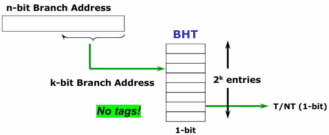
The Branch History Table (BHT), also referred to as the Branch Prediction Buffer, is a simple yet effective mechanism used in dynamic branch prediction. It consists of a table where each entry holds a single bit representing the most recent outcome of a branch—either taken or not taken.
The primary purpose of the BHT is to provide a fast, hardware-based prediction that can be used to determine the likely direction of a branch instruction before it is fully resolved in the pipeline.
Each entry in the table is indexed using the lower-order bits of the branch instruction address, ensuring a compact design while leveraging the principle of locality in programs—where nearby instructions tend to execute together.
Importantly, the table does not contain tags, meaning that every lookup results in a "hit."
This also implies that different branches with the same lower-order address bits may share an entry, leading to occasional inaccuracies. However, since branch prediction is merely a hint rather than an absolute decision, these minor errors are acceptable within the broader goal of improving pipeline efficiency.
1-Bit Branch History Table
In its simplest form, the BHT maintains a single-bit prediction per branch. The prediction is used to speculatively execute instructions along the predicted path. If the prediction is correct, execution continues without interruption. However, if the prediction is incorrect, the pipeline must be flushed, the prediction bit is inverted, and execution resumes from the correct instruction, incurring a one-cycle penalty.
One major weakness of the 1-bit BHT arises when dealing with loop branches. In a typical loop, the branch is taken for most iterations but is not taken when exiting the loop. This behavior leads to two mispredictions per loop execution:
At the last iteration: The predictor assumes the branch is taken, but the program exits the loop.
At the first iteration of the next execution: Since the previous misprediction caused the predictor to flip to not taken, it incorrectly predicts that the branch will not be taken, leading to another misprediction.
Example
For example, in a loop with 10 iterations, where the branch is taken 9 times and not taken once, a 1-bit BHT results in an 80% accuracy rate (eight correct predictions and two mispredictions).
2-Bit Branch History Table
To address the instability of the 1-bit BHT, processors often implement a 2-bit Branch History Table, which provides a more refined state transition mechanism. Instead of immediately flipping the prediction bit after a single misprediction, the 2-bit BHT encodes four states, requiring two consecutive mispredictions before changing the prediction:
Strongly Taken (predict taken, remains taken unless mispredicted twice).
Weakly Taken (predict taken, but changes to not taken after one misprediction).
Weakly Not Taken (predict not taken, but changes to taken after one misprediction).
Strongly Not Taken (predict not taken, remains not taken unless mispredicted twice).
This structure allows the predictor to maintain stability in loop branches, where the branch is usually taken. With a 2-bit BHT, the last iteration of a loop still results in a misprediction, but the prediction does not immediately flip to not taken. Consequently, when the loop begins again, the predictor still predicts taken, avoiding the second misprediction.
Example
For the same 10-iteration loop example, a 2-bit BHT results in a 90% accuracy rate, since only one misprediction occurs (at the final loop iteration).
Correlating Branch Predictors
The 2-bit Branch History Table (BHT), while effective in reducing mispredictions, operates under the assumption that a branch’s past behavior is the best predictor of its future behavior. However, in many real-world programs, the behavior of one branch can be influenced by the outcome of other recently executed branches. This phenomenon, known as branch correlation, suggests that tracking only the history of a single branch may be insufficient for accurate prediction.
To address this limitation, modern processors employ Correlating Branch Predictors, also known as Two-Level Predictors. These predictors extend the traditional BHT approach by incorporating the history of multiple recently executed branches to improve prediction accuracy. Instead of using just the outcome of the current branch, these predictors track patterns across multiple branches, leveraging the interaction between consecutive branch instructions to refine future predictions.
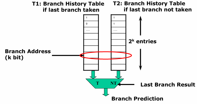
A Correlating Branch Predictor maintains a record of whether recently executed branches were taken or not taken. When predicting the outcome of a new branch, the predictor selects an appropriate Branch History Table (BHT) based on this past behavior. Specifically:
If the last executed branch was taken, the predictor selects a particular BHT for prediction.
If the last executed branch was not taken, a different BHT is used.
This approach allows the predictor to consider interdependencies between branches, rather than treating each branch in isolation.
Correlating Predictors
A more generalized form of correlation-based prediction is the correlating predictor, where:
represents the number of previous branches tracked.
refers to the number of bits used for prediction per entry in the BHT.
This means that the last branches’ outcomes are used to determine which of the possible BHTs should be used for prediction. The indexing mechanism typically involves concatenating low-order bits of the branch address with an -bit global history of recently executed branches, ensuring that the predictor adapts dynamically to execution patterns.
Two-Level Adaptive Branch Predictors
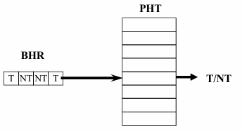
A more advanced refinement of correlating predictors is the Two-Level Adaptive Branch Predictor, which introduces two distinct components:
Branch History Register (BHR)
A -bit shift register that records the outcomes of the last executed branches.
This acts as a global history that captures recent execution trends.
Pattern History Table (PHT)
A table of 2-bit saturating counters, which stores prediction information for specific branch history patterns.
The BHR acts as an index into the PHT, selecting the appropriate 2-bit counter for prediction.
Once the counter is selected, the branch is predicted using the same mechanism as the standard 2-bit counter scheme (i.e., increasing or decreasing the counter based on the actual outcome).
By combining local and global history tracking, Two-Level Adaptive Predictors achieve a more refined and context-aware prediction mechanism. They are particularly effective in scenarios where the outcome of a branch is influenced by the behavior of multiple preceding branches, such as nested loops and conditional branches in complex execution flows.
While traditional branch prediction methods like the 2-bit BHT provide moderate accuracy, they fail to capture correlations between different branches. Correlating Branch Predictors overcome this limitation by incorporating the history of multiple past branches into their prediction model, significantly improving accuracy in complex branching scenarios. The Two-Level Adaptive Predictor further enhances prediction by introducing a hierarchical structure, where a Branch History Register records global trends, and a Pattern History Table refines predictions using local information.
GA Predictor and GShare Predictor
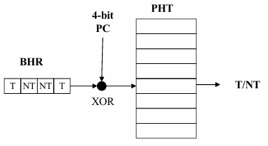
The Global 2-Level Predictor is a branch prediction technique that enhances accuracy by utilizing the correlation between the current branch and other branches within the global history. The underlying mechanism of this predictor is structured around two levels: the Pattern History Table (PHT) and the Branch History Register (BHR). The PHT holds local history information, while the BHR captures the global history of recent branches. The global history is used to index into the PHT, forming the basis for making predictions about the branch outcome.
A variation of the Global 2-Level Predictor is the GShare Predictor, which further refines this mechanism. The key difference between the GA predictor and the GShare predictor is that the GShare correlates the global history (recorded by the BHR) with the low-order bits of the branch address. Specifically, the GShare Predictor performs an XOR operation between the 4-bit BHR and the 4 least significant bits of the program counter (PC), which contains the branch address. This XOR operation creates a unique index into the PHT, allowing the predictor to consider both the global history of branches and the specific location of the current branch in the program, leading to more accurate predictions.
The GShare technique is particularly useful in situations where the outcomes of branches are influenced by both the execution history of recent branches (global history) and the memory address of the current branch. By combining these two factors, the GShare Predictor improves prediction accuracy, especially in complex branching scenarios where single-level predictors may fail to capture the nuances of the program’s flow.
Branch Target Buffer (BTB)
The Branch Target Buffer (BTB), also known as the Branch Target Predictor, is another important component of modern branch prediction mechanisms. Its primary function is to store the Predicted Target Address (PTA) for branches that are predicted to be taken. The PTA is the address where the processor should fetch the next instruction if the branch is indeed taken, and it is typically expressed as PC-relative.
The BTB is designed as a direct-mapped cache that is accessed during the Instruction Fetch (IF) stage of the pipeline. The address of the branch instruction is used to index the cache, and the associated tags are then used for an associative lookup to determine if there is a match in the buffer.
The process begins with the Branch Address Tags, which are derived from the address of the branch instruction. These tags are used to index into the BTB, where the Predicted Target Address (PTA) for the branch is stored. If the index matches an entry in the BTB, it results in a hit, and the PTA is used to continue the fetch process from the predicted branch target. If the branch is not taken, the processor will proceed to the next sequential instruction by using the PC+4 address, which simply advances to the next instruction in memory.
The BTB helps reduce the delay associated with branching by allowing the processor to fetch the next instruction from the predicted target address without waiting for the branch outcome to be fully resolved. This predictive behavior is crucial in maintaining high instruction throughput, especially in highly pipelined and superscalar processors.
The operation of the Branch Target Buffer follows a detailed flowchart that highlights several key steps:
Steps
Branch Address Tags: The branch instruction’s address is used to generate tags that will index into the BTB.
Indexing: The index is derived from these branch address tags and is used to access the cache.
Tags of Branch Address & Predicted Target Address (PTA): The cache contains two columns—one for Branch Address Tags and one for Predicted Target Addresses. These columns are used in an associative lookup to check if the current branch address matches any stored tag.
Hit Determination: If a match (hit) occurs, the system retrieves the Predicted Target Address (PTA) for the branch.
Branch History Table: In some cases, the Branch History Table (BHT) is used to further refine predictions. This table records the historical outcomes (Taken or Not Taken) of previous branches and assists in predicting future outcomes.
Outcome Decision: If the branch is predicted to be taken (a hit in the BTB), the processor fetches instructions from the PTA. If the branch is not taken, it proceeds with the next sequential instruction (PC+4).
This process helps to reduce the penalty associated with branch instructions by preemptively fetching the next instruction from the predicted target address, significantly improving the flow of instruction execution and reducing delays caused by branching decisions.