Numerous challenges in the real world can be effectively modeled and resolved as search problems. This computational paradigm involves an agent exploring various sequences of actions to discover a path from an initial state to a desired goal state. Such an agent, known as a problem-solving agent, engages in a computational process called search when the optimal action is not immediately apparent, necessitating a degree of foresight and planning. These agents typically employ atomic representations, wherein each state of the world is treated as an indivisible entity without any visible internal structure.
The methodology employed by problem-solving agents can be systematically broken down into a four-phase process.
Steps
The first phase is goal formulation, where the agent establishes a specific objective, such as reaching the city of Bucharest from Arad. This step is critical as it narrows the scope of actions to be considered.
The second phase, problem formulation, involves creating an abstract model of the world by defining the states and actions necessary to achieve the formulated goal.
Following this, the agent enters the search phase, where it simulates various action sequences within its abstract model to find one that leads to the goal. A sequence that successfully reaches the goal is termed a solution.
Finally, in the execution phase, the agent carries out the actions prescribed by the solution in the real world.
This approach is most effective in environments that are fully observable, deterministic, static, discrete, and known, as the agent can reliably predict the outcomes of its actions, ensuring that a valid solution found in the model will succeed in reality.
Beyond classic puzzles like the 8-puzzle, this problem-solving framework is applied to a wide array of complex, real-world tasks. Examples include route-finding for navigation systems, intricate airline travel planning, solving touring problems like the Traveling Salesperson Problem (TSP), and highly technical challenges such as VLSI layout design for microchips.
The 8-Puzzle
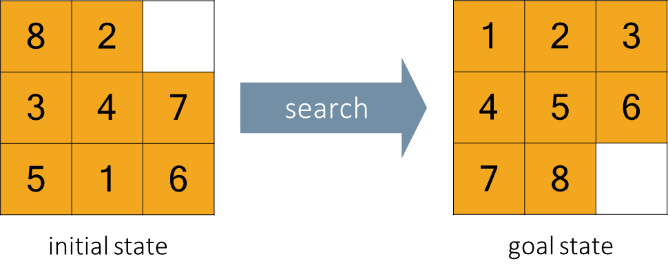
To apply search algorithms, a problem must first be formally defined. This formalization provides the necessary structure for an agent to reason about states and actions. The 8-Puzzle, a variant of the sliding-tile puzzle on a grid, serves as a classic example for illustrating this process. The objective is to transition from a given initial configuration of tiles to a specified goal configuration by sliding tiles into the empty space.
A problem is formally defined by five components: the state space, an initial state, the available actions, a transition model, and a goal test, often supplemented by a path cost function.
States and the State Space
Definition
A state is a complete description of a possible arrangement of the environment.
For the 8-Puzzle, a state is defined by the specific location of each of the eight numbered tiles and the single blank space on the grid. The collection of all possible valid configurations constitutes the state space of the problem.
The agent begins in a designated initial state and performs a search through the state space to find a path to one or more goal states. For the 8-puzzle, a typical goal state is having the tiles arranged in numerical order.
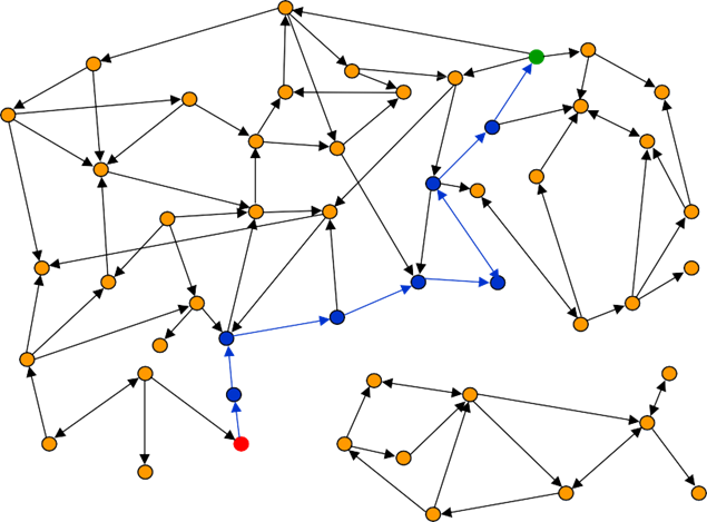
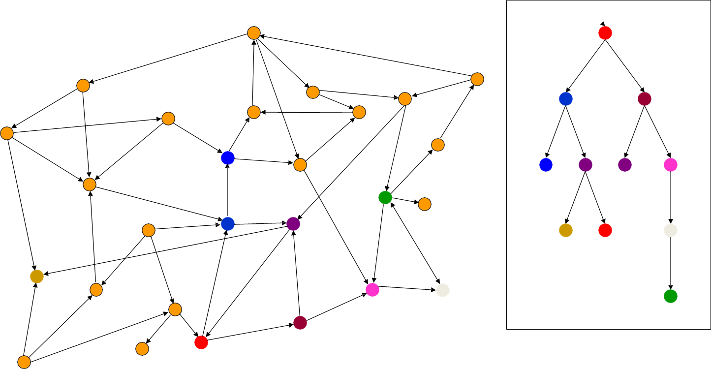
The state space can be visualized as a directed graph where each node represents a state, and each directed edge represents an action that transitions from one state to another. A path in this graph is a sequence of states connected by actions. There is an arc from state to state if and only if is a successor of .
The solution to the problem is a path in the state space from the initial state to a goal state, a particular state that satisfies the goal test.
Actions
Definition
For any given state , a set of actions defines the possible transitions. The function returns this set of applicable actions.
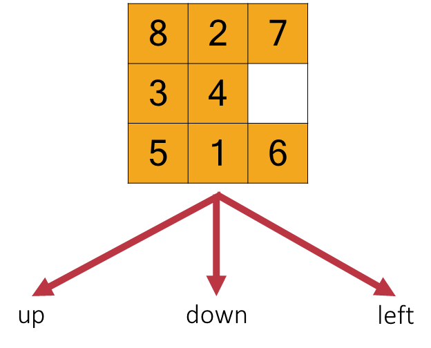
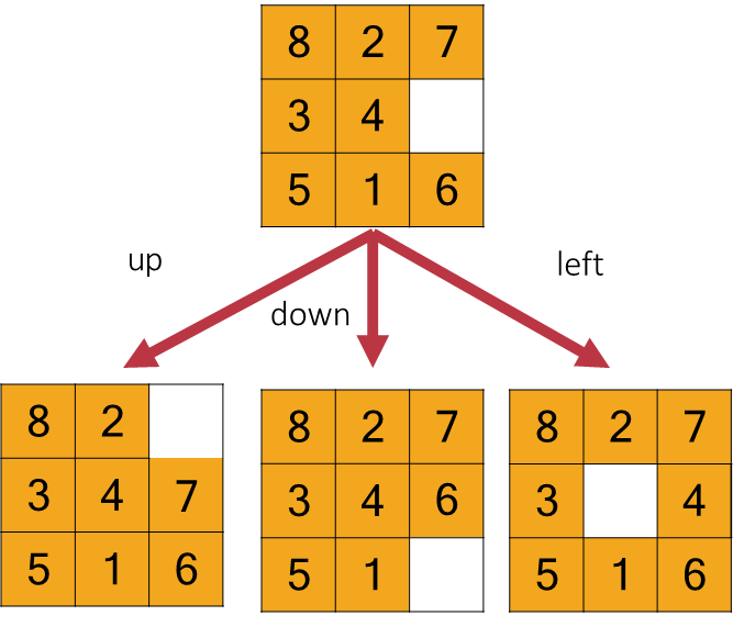
In the context of the 8-Puzzle, the most effective abstraction is to define actions as “movements of the blank space” rather than the individual tiles. Consequently, from any given state, the blank space can be moved Left, Right, Up, or Down, provided it is not at an edge or corner that would make one or more of these movements impossible.
The Transition Model and Path Cost
Definition
The transition model specifies the outcome of performing an action in a particular state. This is often represented by a function, , which returns the new state that results from executing action in state .
For instance, if the action Right is applied to a state where the blank is to the left of the ‘5’ tile, the resulting successor state will have the blank and ‘5’ tile positions swapped.
Accompanying the transition model is the action cost function, denoted as , which assigns a numeric cost to performing action to transition from state to . For the standard 8-Puzzle, each move has a uniform cost of 1. The total cost of a solution is the sum of the individual action costs along the path from the initial state to the goal state.
An optimal solution is one that has the lowest path cost among all possible solutions.
The Challenge of Scale
In practice, explicitly constructing and storing the entire state-space graph is often infeasible due to its immense size. The number of states can grow exponentially with the complexity of the problem.
the state space for the game of Chess is estimated to be as large as .
In general, consider the -puzzle problem and suppose to generate millions states per second, it would require seconds to generate the 8-puzzle state space, less than 4 hours for the 15-puzzle, and more than years for the 24-puzzle. There is also a memory issue: the number of states in the game of chess is estimated to be between and , while the number of states in the game of Go is around . For context, the estimated number of atoms in the observable universe is between and .
Some problems even feature infinite state spaces, such as one conceived by Donald Knuth where operations like square root, floor, and factorial can be applied to numbers, generating an endless sequence of new states. This colossal scale means that a problem-solving agent cannot simply build the entire graph and then search it; it must find a solution by exploring only a tiny fraction of the total state space.
The Importance of Problem Formulation
The process of removing unnecessary detail from a representation is known as abstraction. How a problem is formulated through abstraction has a profound impact on the difficulty of the search. A good problem formulation captures all necessary information while omitting irrelevant details that would needlessly expand the state space.
For example, when planning a driving route from Arad to Bucharest, the model can abstract away details like the weather, the radio program, or the scenery, as they are irrelevant to finding a path.
An effective abstraction is one where the abstract actions, like “drive from Arad to Sibiu,” are easier to carry out than the original problem itself.
The Eight-Queens Puzzle
The Eight-Queens puzzle requires placing eight queens on a chessboard such that none can attack another.
A naive formulation where states are any arrangement of 0 to 8 queens yields a state space of approximately ; in this formulation, the function allows placing a queen in any empty square, leading to an enormous number of possible configurations.
A much better formulation enforces the constraint that each queen must be in a different column. In this version, actions involve placing a queen in the leftmost empty column in a square that is not attacked by existing queens. This superior formulation reduces the state space to a mere states, making the problem vastly more tractable.
Path Planning
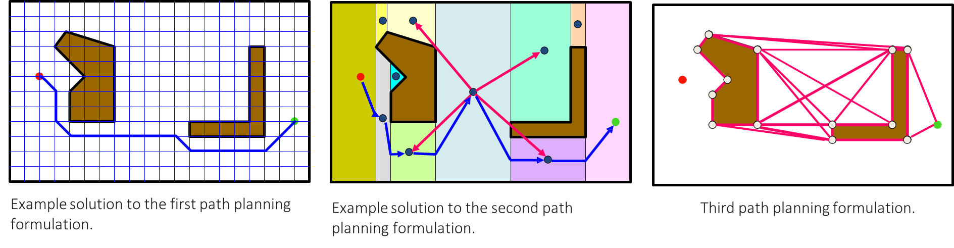
For finding a path in a 2D space with obstacles, different formulations offer various trade-offs.
A grid-based approach discretizes the world, making it simple but potentially coarse.
A cell decomposition method divides the space into convex polygons, offering a more structured representation.
A visibility graph, where states are the start, goal, and obstacle vertices, and actions are straight-line movements to visible vertices, is capable of finding the shortest possible path.
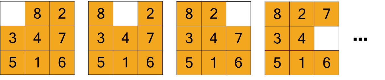
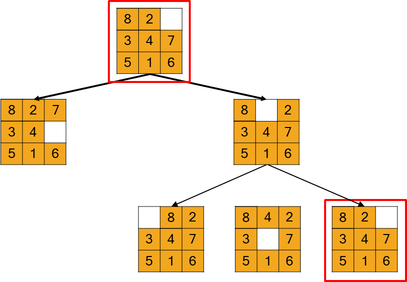
From State Space to Search Tree
Search algorithms find solutions by superimposing a search tree over the state-space graph. The process begins at the root of the tree, which corresponds to the initial state. The algorithm then progressively explores paths by expanding the current node, which involves generating a child node for each state that can be reached by applying a valid action. This continues until a node corresponding to a goal state is generated.
Search Tree vs. State Space
It is critical to distinguish between the state space and the search tree.
The state space describes the complete set of states and transitions in the world.
In contrast, the search tree describes specific paths from the initial state toward the goal.
A single state can be represented by multiple nodes in the search tree if there are different paths to reach it. This distinction is important because, in problems with cycles (or “loopy paths”), the search tree can become infinite even if the state space is finite, as an algorithm could repeatedly traverse a loop without end.
The Node Data Structure
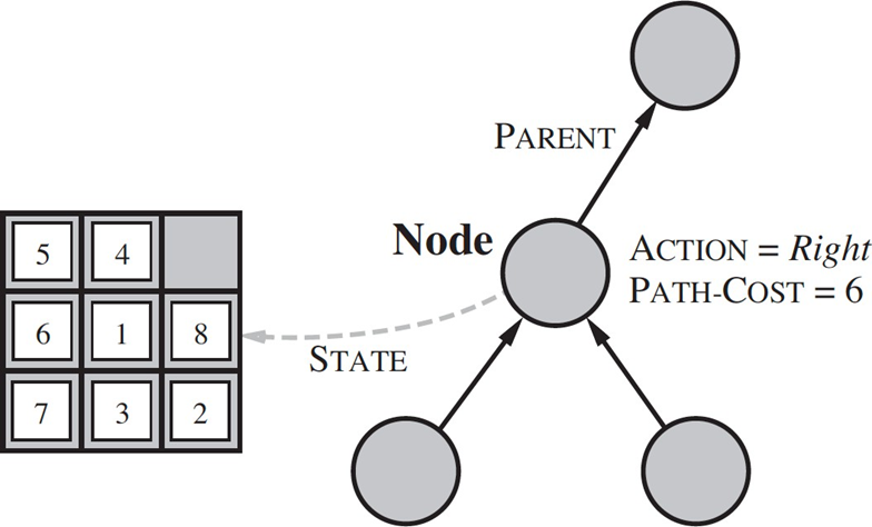
A search tree is composed of nodes, which are data structures containing several key pieces of information. Each node includes node.STATE, the state in the state space to which the node corresponds. It also contains node.PARENT, a pointer to the node that generated it, which is essential for reconstructing the solution path once a goal is found. The node stores node.ACTION, the action applied to the parent’s state to create this node, and node.PATH-COST (also denoted as ), which is the total cost of the path from the initial state to
The depth of the node, or the number of steps from the root, can also be stored.
class Node:
    def __init__(self, state, parent=None, action=None, path_cost=0):
        """Create a search tree Node, derived from a parent by an action."""
        self.state = state
        self.parent = parent
        self.action = action
        self.path_cost = path_cost
        self.depth = 0
        if parent:
            self.depth = parent.depth + 1
Generic Tree-Search Algorithms
The fundamental process of finding a solution in a state space can be described by a generic tree-search algorithm.
Algorithm
This process begins by initializing a search tree with a root node corresponding to the problem’s initial state. The algorithm then enters a loop where it iteratively selects a node for expansion from a set of generated but not-yet-expanded nodes.
Initialize the root of the tree with the initial state of problem

LOOP DO
	IF there are no more nodes candidate for expansion THEN
		RETURN failure

	select a node not yet expanded

	IF the node corresponds to a goal state THEN
		RETURN the corresponding solution
	ELSE expand the chosen node, adding the resulting nodes to the tree
This collection of nodes is known as the frontier. If the frontier becomes empty before a solution is found, the algorithm has failed to find a solution and terminates. Otherwise, it selects a node, checks if its corresponding state is a goal state, and if so, returns the solution path. If it is not a goal, the node is expanded by applying all valid actions to its state to generate a set of child nodes, which are then added to the frontier.
The specific search strategy is determined by the order in which nodes on the frontier are selected for expansion.
def expand(self, problem) : """ List the nodes reachable in one step from this node. """ return [self.child node(problem, action) for action in problem.actions(self.state) ]def child_node (self, problem, action) : next_state = problem.result(self.state, action) next_node = Node(next_state, self, action, problem.path_cost(self.path_cost, self.state, action, next_state) ) return next_node
The frontier itself can be conceptualized as a separator between two regions of the state-space graph: an interior region of states corresponding to nodes that have already been expanded, and an exterior region of states that have not yet been reached.
Handling Redundancy with Graph Search
A simple search algorithm that does not keep track of previously visited states, known as a tree-like search, can be highly inefficient. In state spaces where actions are reversible, such as in the 8-puzzle or robot navigation, the algorithm may waste significant effort exploring redundant paths, which are simply worse ways to get to an already-visited state. This can lead to the generation of a search tree that is infinite in size, even for a finite state space, as the algorithm can get trapped in cycles, or loopy paths.
For example, a path from Arad to Sibiu and back to Arad is a cycle that accomplishes nothing but increases the path length.
To mitigate this, a more sophisticated approach called graph search is used.
initialize the root of the tree with the initial state of problem
initialize the reached list to the empty set

LOOP DO
	IF there are no more candidate nodes for expansion THEN
		RETURN failure

	choose a node not yet expanded

	IF the node corresponds to a goal state THEN
		RETURN the corresponding solution

	Expand the chosen node into a list of child nodes

	For each child node,
		IF the state of the child node is not in the reached list OR the path cost of the child node is lower than the cost of the reached list node THEN
			add/update the reached list with the child node information add the child node to the tree
This method maintains a data structure, often a lookup table or hash table, to store all states that have been reached. When a new child node is generated, the algorithm checks if its state has been reached before. If the state is new, the node is added to the frontier. If the state has been reached previously, the new node is only added if the path to it is cheaper than the previously discovered path. This ensures that the algorithm always finds the most efficient path to any given state while avoiding the redundant exploration of cycles and longer paths.
Problem Type
Repeated States?
Search Tree Size
8 Queens
No (only add queens)
Finite
Assembly Planning
Few (usually no cycles)
Finite
8-Puzzle
Many (reversible moves)
Infinite (with Tree-like Search)
Robot Navigation
Many (can move back and forth)
Infinite (with Tree-like Search)
Best-First Search
Best-first search is a general and powerful instance of a graph search algorithm that provides a framework for various specific strategies. It operates by selecting a node from the frontier that has the minimum value according to an evaluation function, . The frontier is maintained as a priority queue, which is ordered according to these -values, ensuring that the most promising node is always chosen for expansion first.
function BEST-FIRST-SEARCH(problem,f) returns a solution node or failure
	node ← NODE(STATE=problem.INITIAL)
    frontier ← a priority queue ordered by f, with node as an element
    reached ← a lookup table, with one entry with key problem.INITIAL and value node

    WHILE not IS-EMPTY(frontier) DO
  	    node ← POP(frontier)

  	    IF problem.IS-GOAL(node.STATE) THEN return node

  	    FOR EACH child in EXPAND(problem, node) DO
	  		st ← child.STATE

	  		IF s is not in reached OR child.PATH-COST < reached[s].PATH-COST THEN
	  			reached[s] ← child
		        add child to frontier

  	RETURN failure

function EXPAND(problem, node) yields nodes
  s ← node.STATE

  FOR each action in problem.ACTIONS(s) DO
    s' ← problem.RESULT(s, action)
    cost ← node.PATH-COST + problem.ACTION-COST(s, action, s')
    yield NODE(STATE=s', PARENT=node, ACTION=action, PATH-COST=cost)
The algorithm begins with the initial state in the frontier and an empty set of reached states. On each iteration, it removes the node with the lowest -value from the priority queue. If this node’s state is a goal, the algorithm returns the corresponding solution. Otherwise, the node is expanded, and for each resulting child node, its state is checked against the set of reached states. A child node is added to the frontier only if its state has not been reached before, or if this new path to the state has a lower path cost than any previously recorded path to that same state. This ensures that the algorithm systematically explores the state space while avoiding redundant paths and prioritizing nodes that appear to be closest to a solution.