In our study of artificial intelligence, we began by treating search problems as abstract entities.
Definition
A standard search problem is defined by a “black box” state representation. The internal structure of a state is arbitrary and opaque to the search algorithm. The algorithm can only perform a few simple operations:
- Test if a state is a goal state.
- Generate the successor states from a given state.
General-purpose search algorithms like Breadth-First Search (BFS), Depth-First Search (DFS), and A* are designed to work on any such problem. While this generality is powerful, it can be inefficient. The algorithms lack deeper insight into the problem’s nature, treating states as indivisible wholes.
However, many problems have inherent structure. If we can specialize the problem representation to expose this structure, we can design more sophisticated and efficient search algorithms. This specialization may narrow the class of problems we can solve with a particular algorithm, but the gain in performance for that class is often substantial. Constraint Satisfaction Problems (CSPs) represent a pivotal step in this direction, moving from opaque states to states with a factored representation.
It’s crucial to distinguish between two primary motivations for searching:
- Planning Problems: In these problems, the solution is the path from an initial state to a goal state. The goal is to find a sequence of actions that achieves a desired outcome. The path itself is the valuable output.
The 8-puzzle or 15-puzzle (the solution is the sequence of moves), navigation and route planning (the solution is the route to take).
Paths have varying costs and depths, and problem-specific heuristics (like Manhattan distance) are used to guide the search for an optimal path.
- Identification Problems: In these problems, the solution is the goal state itself, not the path to reach it. The objective is to find a configuration of the world that satisfies a set of requirements. For many formulations of these problems, all valid solutions are found at the same depth in the search tree.
The 8-Queens problem (the solution is a valid placement of 8 queens on a chessboard), Sudoku, designing a floor plan.
The goal state is the primary focus. The search is for a valid assignment of values to variables.
Constraint Satisfaction Problems (CSPs)
Constraint Satisfaction Problems (CSPs) are a specialized, powerful framework for solving identification problems. A CSP is defined by a simple, structured set of components. This structure is the key to its power.
Definition
A Constraint Satisfaction Problem consists of three main elements:
- Variables (
): A set of variables, . Each variable represents a part of the problem that needs a value assigned to it. - Domains (
): A set of domains, , where is the finite set of possible values for the variable . - Constraints (
): A set of constraints, . Each constraint specifies the allowable combinations of values for a subset of the variables.
A state in a CSP is a partial or complete assignment of values to variables. A solution is a complete and consistent assignment.
- Complete: Every variable in
is assigned a value from its domain. - Consistent: The assignment does not violate any of the constraints in
.
The total number of possible complete assignments is the size of the Cartesian product of the domains:
The goal of CSP algorithms is to find a solution without exploring this entire space.
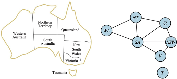
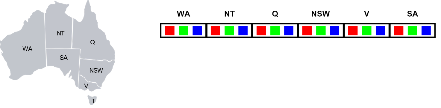
Example: Map Coloring
The map coloring problem is a classic illustration of a CSP.
- Variables: The regions on the map. For Australia:
{WA, NT, Q, NSW, V, SA, T}.- Domains: The set of available colors for each region:
{red, green, blue}.- Constraints: Adjacent regions must have different colors. This translates to a set of binary inequality constraints:
WA ≠ NT,WA ≠ SA,NT ≠ SA,NT ≠ Q,SA ≠ Q,SA ≠ NSW,SA ≠ V,Q ≠ NSW,NSW ≠ V.- Solution: A complete assignment, such as
{WA=red, NT=green, Q=red, NSW=green, V=red, SA=blue, T=green}.

Modeling with CSPs
The CSP framework is versatile and can model a wide variety of real-world problems.
8-Queens Problem
The goal is to place 8 queens on an
chessboard so that no two queens threaten each other.
- Variables:
for , where represents the row of the queen in column . - Domains:
for each variable. - Constraints:
- No two queens on the same row:
for any . - No two queens on the same diagonal:
for any . - The constraint of “no two queens on the same column” is implicitly handled by our choice of variable representation.
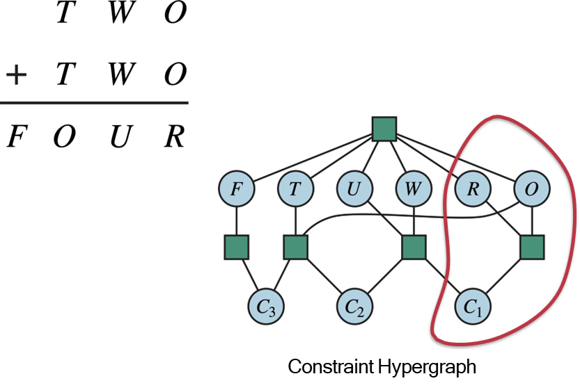
Cryptarithmetic
An arithmetic puzzle where letters represent digits. For example:
TWO + TWO = FOUR.
- Variables: One for each letter
and three carry-over variables . - Domains:
for the letters. for the carry-overs. - Constraints:
- Uniqueness: All letters must have different values. This is a high-order constraint:
Alldiff(F, T, U, W, R, O).- Arithmetic: The columns must sum correctly.
- Leading Zero:
, . The relationships between variables and constraints can be visualized using a Constraint Hypergraph, where nodes are variables and hyperedges connect all variables participating in a single constraint.
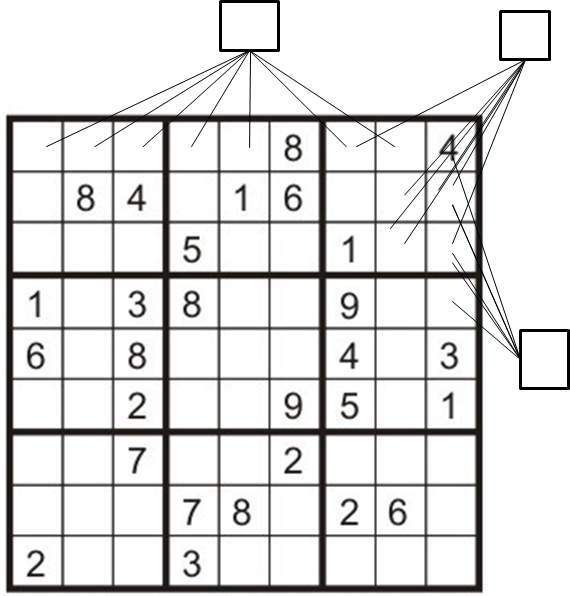
Sudoku
- Variables: One for each of the 81 squares on the grid,
. - Domains:
for each empty square. A single value for pre-filled squares. - Constraints: A 9-way
Alldiffconstraint for each row, each column, and eachbox.
Task Scheduling
- Variables: The tasks to be scheduled, e.g.,
. The variables could represent start times, end times, or durations. - Domains: A range of possible times or time intervals.
- Constraints: Temporal relationships between tasks.
must be done during and . must be completed before starts . must overlap with and . gantt title Task Scheduling Example dateFormat HH:mm axisFormat HH:mm section Tasks T1 :a1, 09:00, 2h T2 :a2, after a1, 1h T3 :a3, 10:00, 3h T4 :a4, after a2, 1h
The Constraint Graph
Most CSPs encountered in practice involve binary constraints—constraints that relate exactly two variables. These are the simplest and most common type, and they allow us to represent the problem using a constraint graph, where:
- Nodes correspond to variables.
- Edges (arcs) connect pairs of variables that share a constraint.
This graphical structure is not just a visualization: it provides valuable information that can be exploited to speed up search and inference.
Example
For instance, in the Australia example, Tasmania (T) is not connected to any other node. This means it is an independent subproblem. We can solve for the mainland and Tasmania completely separately, which drastically reduces the complexity of the search.
Some problems, however, include higher-order constraints involving three or more variables (such as the Alldiff constraint in Sudoku or cryptarithmetic puzzles). Fortunately, any CSP with higher-order constraints can be transformed into an equivalent CSP with only binary constraints through a process called binarization. This transformation enables us to use the powerful techniques and algorithms developed for binary CSPs, leveraging the constraint graph structure for efficient problem solving.
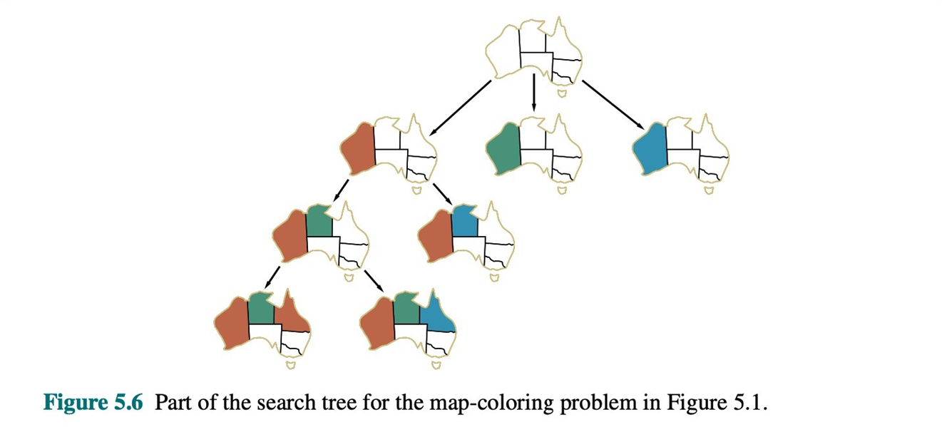
Backtracking Search
The foundational algorithm for solving CSPs is Backtracking Search. It is a form of depth-first search that builds a solution by incrementally assigning values to variables. Its efficiency comes from intelligently pruning branches of the search tree that cannot lead to a solution.
Backtracking search is based on two key principles:
- One Variable at a Time: At each step of the search, we select an unassigned variable and consider all values in its domain. This is valid because variable assignments are commutative—the order in which we assign values does not affect whether the final assignment is a solution.
[WA=red, NT=green]is the same solution as[NT=green, WA=red]. - Check Constraints as You Go: When we consider assigning a value to a variable, we immediately check if that value is consistent with all previously assigned variables. If it violates any constraint, we discard that value and do not explore any deeper down that path. This is effectively an “incremental goal test.”
The Backtracking Algorithm
The pseudocode for the recursive backtracking algorithm is as follows:
function BACKTRACKING-SEARCH(csp) return a solution of failure
  return BACKTRACK(csp, {}) // Start with an empty assignment

function BACKTRACK(csp, assignment) returns a solution or failure
  if assignment is complete then return assignment

  var ← SELECT-UNASSIGNED-VARIABLE(csp, assignment)

  for each value in ORDER-DOMAIN-VALUES(csp, var, assignment) do
    if value is consistent with assignment then
      add {var = value} to assignment
      result ← BACKTRACK(csp, assignment)

      if result != failure then return result

      remove {var = value} from assignment // Backtrack step

  return failure // No value worked for this var
The algorithm explores the search space by picking a variable, trying a value, and then recursively calling itself. If the recursive call leads to a dead end (returns
failure), it backtracks by undoing the assignment and trying the next available value. If all values for a variable lead to failure, it backtracks further up the tree.
Improving Backtracking Performance
The simple backtracking algorithm works, but its performance can be dramatically improved. The plain algorithm makes “dumb” choices about which variables and values to choose, and it is slow to detect failures that are inevitable. The three primary avenues for improvement are:
- Filtering (Constraint Propagation): Can we detect inevitable failures early? By looking ahead at the domains of unassigned variables, we can prune values that will certainly lead to failure later on. Key techniques include Forward Checking and Arc Consistency.
- Ordering: In what order should we process variables and values?
- Variable Ordering: Which variable should be assigned next? Good heuristics can lead to failures being found much earlier, pruning the search tree more effectively.
- Value Ordering: In what order should a variable’s values be tried? A good heuristic can guide the search towards a solution more quickly.
- Structure: Can we exploit the problem’s structure, as seen in the constraint graph, to solve it more efficiently (e.g., by breaking it into independent subproblems)?
These improvements transform backtracking from a simple brute-force method into a highly effective tool for solving complex real-world problems.
Filtering
The core idea of filtering is to move beyond simply checking a new assignment against past assignments. Instead, we propagate the implications of an assignment forward to constrain the possible values of future (unassigned) variables. If we can ever foresee that a current partial assignment will inevitably lead to a situation where a future variable has no legal values left, we can backtrack immediately.
Forward Checking
Forward checking is the simplest form of filtering. It establishes a basic level of “local” consistency.
Idea
When a variable
is assigned a value , the forward checking algorithm immediately looks at each unassigned variable that is connected to by a constraint. For each such , it deletes any value from its domain that is inconsistent with the assignment .
Example: Map Coloring with Forward Checking
Let’s trace this on the Australia map-coloring problem. The initial domains for all variables are
{Red, Green, Blue}.
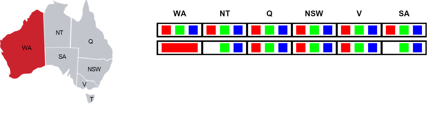
- Assign
WA = Red.
- Forward checking inspects
WA’s neighbors:NTandSA.- It removes
Redfromand . - Resulting Domains:
NT:{Green, Blue}SA:{Green, Blue}- (Others remain
{Red, Green, Blue})
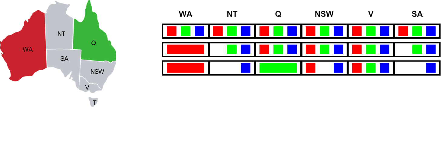
- Assign
Q = Green.
- Forward checking inspects
Q’s neighbors:NT,SA, andNSW.- It removes
Greenfrom, , and . - Resulting Domains:
NT:{Blue}(was{Green, Blue})SA:{Blue}(was{Green, Blue})NSW:{Red, Blue}
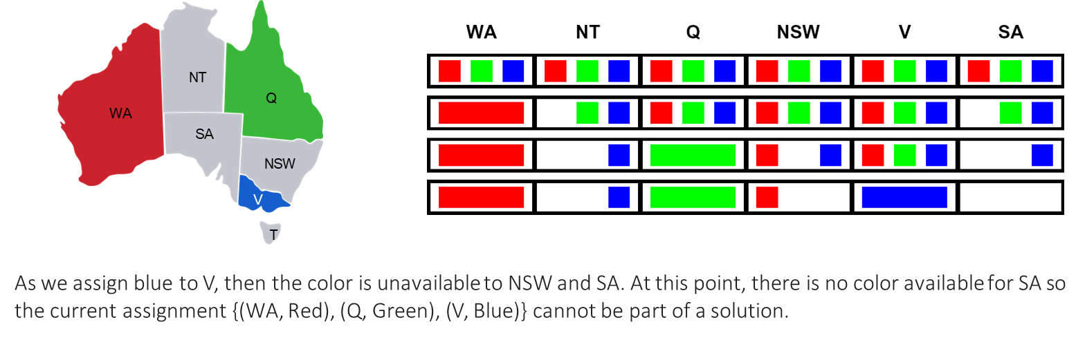
- Assign
V = Blue.
- Forward checking inspects
V’s neighbors:SAandNSW.- It removes
Bluefromand . - Resulting Domains:
SA:{}(was{Blue})NSW:{Red}(was{Red, Blue})
At this point, the domain of
SAhas become empty. Forward checking has revealed that the current partial assignment{WA=Red, Q=Green, V=Blue}cannot possibly be extended to a full solution. The algorithm can therefore backtrack immediately, without needing to try assigning values to any other variables. This early failure detection is the primary benefit of forward checking.
If a problem has
Arc Consistency (AC-3)
Forward checking is useful, but it doesn’t detect all possible inconsistencies. Consider the state after step 2 in the example above: NT’s domain is {Blue} and SA’s domain is {Blue}.
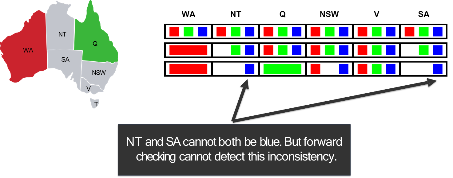
The constraint NT ≠ SA is clearly violated, yet forward checking did not detect this because it only checks constraints between the newly assigned variable (
Arc consistency is a more powerful filtering technique that addresses this.
Definition
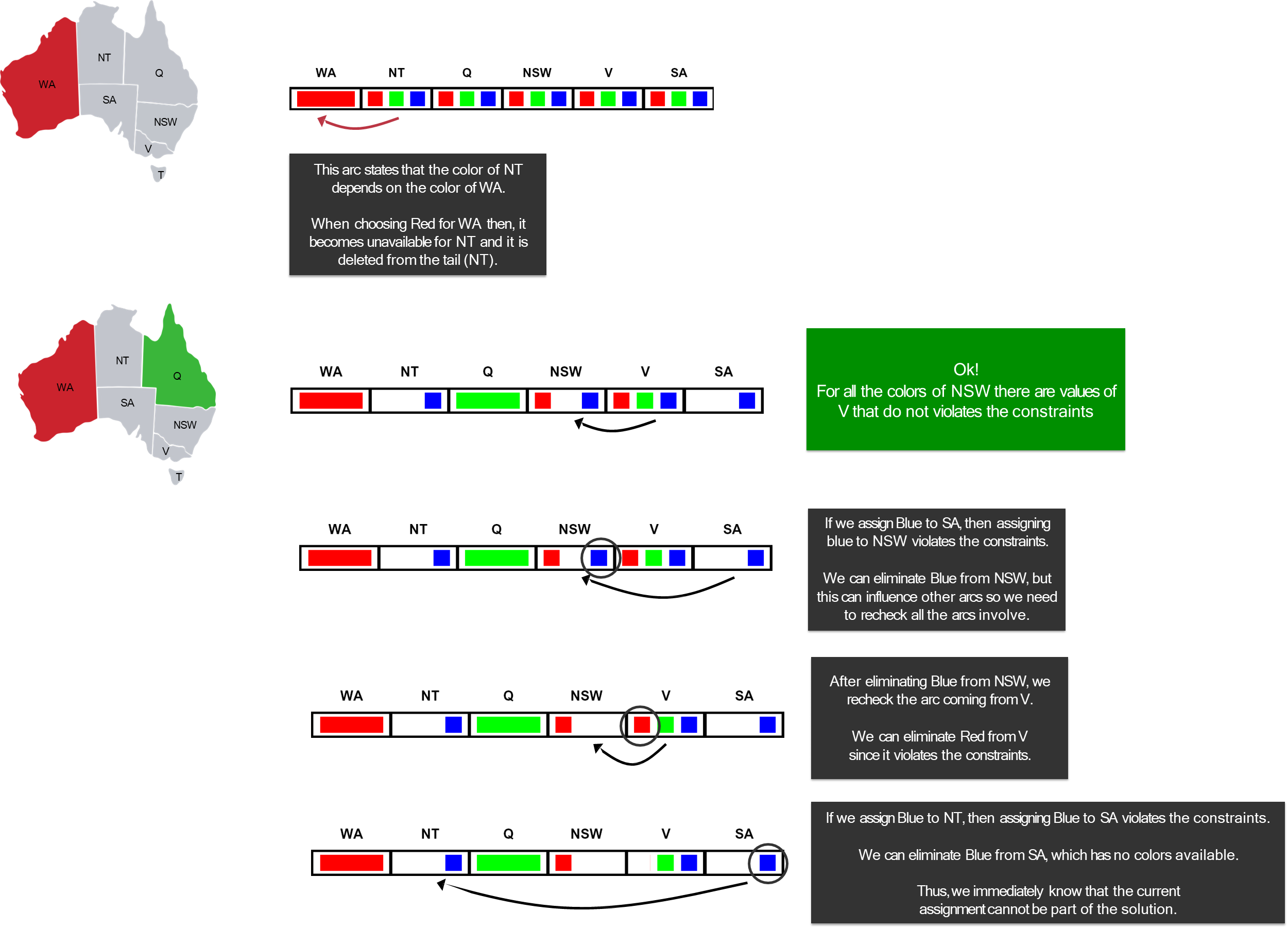
An arc
is considered arc-consistent if for every value in the domain of , there exists at least one value in the domain of such that the assignment is valid. Essentially, every value in the “tail” of the arc (
) must have a “supporting” value in the “head” ( ). If a value in has no supporting value in , then can be safely removed from , as it cannot be part of any consistent solution.
The AC-3 Algorithm
The most common algorithm for enforcing arc consistency is AC-3. It works as follows:
function AC-3(csp) returns false if an inconsistency is found and true otherwise
  queue ← a queue of arcs, initially all the arcs in csp

  while queue is not empty do
    (Xi, Xj) ← POP(queue)

    if REVISE(csp, Xi, Xj) then
      if size of Di = 0 then return false

      for each Xk in Xi.NEIGHBORS − {Xj} do
        add(Xk, Xi) to queue
  return true

function REVISE(csp, Xi, Xj) returns true iff we revise the domain of Xi
  revised ← false

  for each x in Di do
    if no value y in Dj allows (x, y) to satisfy the constraint between Xi and Xj then
      delete x from Di
      revised ← true
  return revised
- Initialize a queue containing all the arcs in the CSP (for every binary constraint
, both and are added). - While the queue is not empty:
- Dequeue an arc,
. - For each value
in , check if there is a corresponding value in that satisfies the constraint. - If a value
has no such support in , remove from . - If any value was removed from
(i.e., its domain was revised), then for every neighbor of (other than ), add the arc back to the queue. This is the crucial propagation step: a change in may cause inconsistencies in other arcs pointing to it, so they must be re-checked. - The algorithm terminates when the queue is empty (all arcs are consistent) or if any domain becomes empty (proving no solution exists).
AC-3 can be run as a preprocessing step before search begins, or it can be interleaved with backtracking search (a strategy known as Maintaining Arc Consistency, or MAC). It is more computationally expensive than forward checking—with complexity
Ordering Heuristics
Filtering helps prune the search tree by eliminating bad choices. Ordering heuristics help by guiding the search toward good choices first. These heuristics are domain-independent and rely solely on the factored structure of the CSP. They answer two fundamental questions at each step of the search.
Summary of Heuristics:
- To select a variable (fail-fast):
- MRV: Pick the variable with the fewest remaining values.
- Degree Heuristic: As a tie-breaker, pick the one affecting the most other unassigned variables.
- To select a value (succeed-fast):
- LCV: Pick the value that prunes the fewest values from the domains of neighboring variables.
Which variable should be assigned next?
The goal here is to find failures as early as possible. This is the “fail-fast” principle. By identifying a dead-end early, we prune the entire subtree below it.
-
Minimum Remaining Values (MRV):
- Rule: Choose the variable that has the fewest legal values left in its domain.
- Intuition: This is also known as the “most constrained variable” heuristic. A variable with only one or two remaining values is a critical bottleneck. By selecting it, we quickly test the most difficult part of the problem. If it has no valid assignment, we fail immediately. If we were to choose a variable with many values, we might explore a long, fruitless path before discovering the bottleneck variable had no solution.
-
Degree Heuristic (DH):
- Rule: Choose the variable that is involved in the largest number of constraints with other unassigned variables.
- Intuition: This heuristic is primarily used as a tie-breaker for MRV. The idea is to choose a variable that, once assigned, will have the greatest impact on constraining the rest of the problem. This helps to prune future choices more effectively and reduce the size of the subsequent search space.
The standard strategy is to use MRV, and then use DH to break ties.
In what order should its values be tried?
Once a variable is selected, we must decide the order in which to try its values. Here, the strategy is the opposite of fail-fast. We want to “succeed-fast” by picking a value that is most likely to be part of a solution.
- Least Constraining Value (LCV): ^LCV
- Rule: Prefer the value that rules out the fewest choices for the neighboring unassigned variables.
- Intuition: This heuristic tries to maintain maximum flexibility for the rest of the search. By picking a value that leaves the most options open for its neighbors, we increase the chances of finding a solution without having to backtrack.
Exploiting Problem Structure
Beyond filtering and ordering heuristics, the global structure of a CSP, as visualized by its constraint graph, can offer profound opportunities for simplification and dramatic reductions in search complexity.
The most straightforward structural property is the presence of independent subproblems.
Property
An independent subproblem corresponds to a connected component in the constraint graph. A connected component is a set of variables where each variable is connected to at least one other variable in the set, but is not connected to any variable outside the set.
If a problem with
- Without decomposition: The worst-case complexity is
. - With decomposition: We solve
smaller problems. The total cost is .
This shift from an exponential dependency on
Example
Let’s consider a hypothetical large-scale problem:
variables, , (i.e., four subproblems of 20 variables each).
- Without decomposition: The number of assignments to check is
, which would take billions of years on a fast computer. - With decomposition: The cost is
. This is roughly , which can be solved in a fraction of a second.
The Complete Backtracking Algorithm with Improvements
We can now synthesize all the techniques—filtering, ordering, and structure (though structure is often handled as a preprocessing step)—into a single, powerful backtracking algorithm. This is often referred to as backtracking search with inference or Maintaining Arc Consistency (MAC).
function BACKTRACKING-SEARCH(csp) a solution or failure
  return BACKTRACK(csp, {})


function BACKTRACK(csp, assignment) return a solution or failure
  if assignment is complete then return assignment

  var ← SELECT-UNASSIGNED-VARIABLE(csp, assignment) // Use MRV and Degree Heuristic

  for each value in ORDER-DOMAIN-VALUES(csp, var, assignment) do // Use LCV
    if value is consistent with assignment then
      add {var = value} to assignment

      // Apply filtering (e.g., AC-3 or Forward Checking)
      inferences ← INFERENCE(csp, var, assignment)

      if inferences ≠ failure then
        add inferences to csp // Temporarily update domains
        result ← BACKTRACK(csp, assignment)

        if result ≠ failure then return result

        // If we reach here, either the value was inconsistent,
        // the inference failed, or the recursive call failed.
        // We must undo everything done in this iteration.
        remove {var = value} from assignment
        remove inferences from csp // Restore domains

  return failure
SELECT-UNASSIGNED-VARIABLE: Implements the MRV and Degree Heuristic.ORDER-DOMAIN-VALUES: Implements the Least Constraining Value heuristic.INFERENCE: This is the crucial new step. After making a tentative assignment, this function applies a filtering algorithm like Forward Checking or AC-3. If filtering causes any variable’s domain to become empty, it returnsfailure, and the algorithm backtracks immediately. Otherwise, it returns the set of domain reductions (“inferences”) it made.
This combined algorithm is the modern workhorse for solving CSPs. It intelligently navigates the search space by making smart choices and pruning branches as early as possible.
A Complete Example: The 4-Queens Problem
Let’s trace this advanced algorithm on the 4-Queens problem.
Variables:
(the column positions of queens in rows 1 to 4). Domains:
for all.
- Initial State:
assignment = {}. AC-3 is run initially, but it removes no values.- Select Variable: All variables have 4 values (MRV tie) and are connected to 3 others (DH tie). We pick
arbitrarily. - Select Value: All values are equivalent. We pick
. - Inference (Forward Checking):
rules out row 1 and diagonals. becomes . becomes . becomes . - Inference (AC-3): Now, we enforce arc consistency on the remaining variables.
- Consider the arc
. If , can have a value? No, because is on a diagonal and is on a diagonal. Therefore, has no support in . - AC-3 removes
from . becomes . - This change propagates. Now consider
. only has the value . If , it conflicts diagonally with . If , it’s on the same row. So becomes empty. - Failure: AC-3 has caused a domain to become empty. The inference step returns
failure.- Backtrack: The assignment
is removed. - Select New Value: We try the next value for
, which is . - Inference:
- Forward Checking:
becomes , becomes , becomes . - AC-3: Checks arcs.
and seems viable. is reduced to and to . The algorithm propagates and finds no further inconsistencies. - Solution Found: The inference step has already reduced the domains of the remaining variables to single values. The search can proceed to assign
, , without further choices, finding the solution .
Beyond AC-3: Higher-Order Consistency
AC-3 enforces consistency over pairs of variables (arcs). However, it does not detect all inconsistencies.
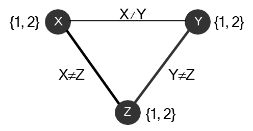
Consider three variables
- This problem is arc-consistent. For any value of
, there is a valid value for . For any value of , there is a valid value for , etc. AC-3 would find no inconsistencies. - However, the problem has no solution. If
, must be . But if , must be . This means and , violating the constraint .
This type of inconsistency can only be found by looking at groups of three variables at a time. This leads to the idea of k-consistency.
- 2-consistency is the same as arc consistency.
- 3-consistency (Path consistency) checks that for any pair of values
for , there exists a value for a third variable such that both constraints are satisfied.
While enforcing higher levels of consistency can prune the search space more, it is also computationally much more expensive. In practice, AC-3 often provides the best compromise between the time spent on inference and the time saved in search.
Search vs. Inference
The power of inference (constraint propagation) raises an interesting point: can some problems be solved without any search at all? The answer is yes.
For some CSPs, running a powerful enough constraint propagation algorithm like AC-3 as a pre-processing step is sufficient to reduce the domain of every variable to a single value. If this happens and no domain becomes empty, that single assignment is the unique solution to the problem.
Example
Many “easy” or “medium” Sudoku puzzles can be solved entirely through logical inference, which is a form of constraint propagation. Techniques like “naked singles” or “hidden singles” are human-friendly names for the results of applying arc consistency and other logic rules. The
CSP-BACKTRACKINGalgorithm, reflects this by first running AC-3 to simplify the problem before even choosing a variable. If the problem is simple enough, the initial AC-3 run might solve it entirely.
This highlights a spectrum in CSP solving:
- Pure Search: Simple backtracking with no inference.
- Interleaved Search and Inference: The MAC algorithm, which is the most common and effective approach.
- Pure Inference: Applying propagation until the problem is solved, with no trial-and-error assignments.
The choice of where to be on this spectrum depends on the specific structure and difficulty of the problem at hand.
A Different Paradigm: Local Search and Optimization
The methods discussed thus far, most notably backtracking search, belong to a class of constructive algorithms. They operate by starting from an empty state and incrementally building a valid configuration, extending a partial solution one variable at a time until a complete and consistent assignment is found.
The philosophy of local search is not to build a solution from scratch, but to refine a complete one. The process begins by generating a complete, though likely invalid, candidate solution, often randomly. From this starting point, the algorithm iteratively applies small, local modifications to move from the current state to a neighboring one. Each step is guided by an objective function, which quantifies the quality of a state. The goal is to make modifications that continually improve this objective value. This process continues until a state is reached from which no further improvement is possible or some other termination criterion, such as a time limit, is met.
A key characteristic of local search is its memorylessness; it operates solely on the
currentstate and does not maintain a history of the path taken or a tree of alternatives.
Hill-Climbing Search
The most elementary form of local search is the hill-climbing algorithm. It is a greedy method that, at every step, chooses the move that yields the greatest immediate improvement in the objective function. To apply hill climbing, a problem must be framed with three components:
- a state representation defining a complete configuration,
- a neighborhood function that generates all states reachable via a single modification, and
- an objective function (or heuristic cost) that assigns a numerical score to every state.
Algorithm
In a maximization context, the algorithm can be described as follows:
function HILL-CLIMBING(problem) returns a state that is a local maximum
  current ← problem.INITIAL

  while true do
    neighbor ← a highest-valued successor state of current

    if VALUE(neighbor) <= VALUE(current) then
      return current

    current ← neighbor
The algorithm relentlessly moves “uphill” until it reaches a “peak”—a state where no neighboring state has a higher value. For minimization problems, the logic is inverted to “valley-descending,” always moving to a neighbor with the lowest cost.
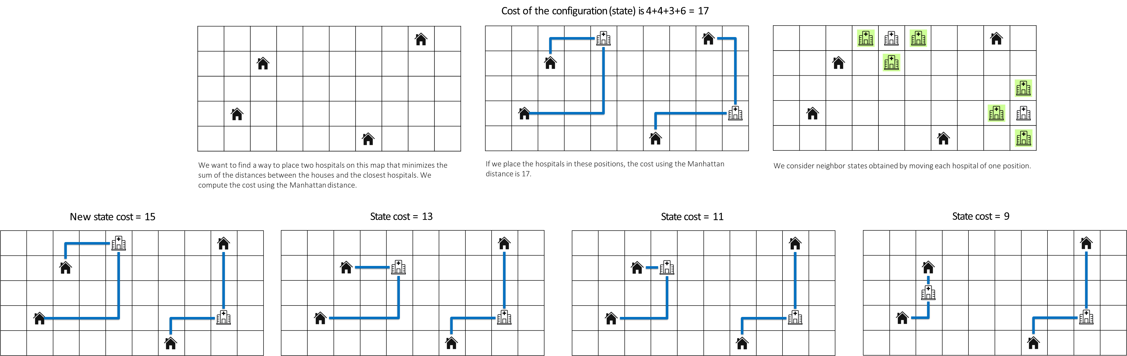
Example
An illustrative example is the Homes and Hospitals problem, an optimization task where the goal is to place two hospitals on a grid to minimize the total Manhattan distance from a set of homes to their respective nearest hospital. A state is a specific placement of the two hospitals. The objective function is the sum of these distances, which is to be minimized. The neighborhood of a state consists of all placements reachable by moving one hospital a single step in any cardinal direction.
A hill-climbing (or, more accurately, valley-descending) search would start from a random hospital placement, repeatedly evaluate all neighboring states, and greedily move to the one that results in the lowest total distance, continuing until no single move can further reduce the cost.
Challenges of the Local Search Landscape
The efficacy of hill climbing is profoundly dependent on the topology of the state-space landscape, an abstract space where each state is a point and its “elevation” is determined by the objective function’s value. The greedy nature of hill climbing makes it susceptible to becoming trapped in suboptimal regions of this landscape, preventing it from discovering the global optimum—the best possible solution.
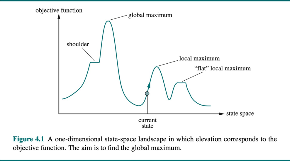
The primary topological challenges include:
- Local Optima: These are states that are superior to all their immediate neighbors but are inferior to the global optimum. A simple hill-climbing algorithm, upon reaching a local optimum, will terminate, as it has no incentive to make a move that would temporarily worsen the objective value.
- Plateaus: These are flat regions in the landscape where neighboring states have the same objective value. In such an area, the algorithm lacks a clear gradient to follow and may either terminate prematurely or wander aimlessly.
- Shoulders: A shoulder is a specific type of plateau from which an upward path does exist, but it is not immediately accessible. The search may be unable to find the direction of ascent from its local neighborhood.
Due to these inherent limitations, more sophisticated local search algorithms, such as random-restart hill climbing (which runs the search multiple times from different random starting points) and simulated annealing (which can accept worsening moves to escape local optima), are often required for complex problems.
Applying Local Search to Constraint Satisfaction Problems
The local search paradigm can be effectively adapted to solve CSPs by reframing them as optimization problems. Instead of searching for a consistent partial assignment, the goal becomes minimizing the number of violated constraints in a complete assignment. This approach, famously implemented in the min-conflicts algorithm, works as follows:
Min-Conflicts Algorithm
- Initialization: Start with a complete, randomly generated assignment of values to all variables (e.g., for the N-Queens problem, place one queen in each column in a random row).
- Objective Function: The cost function,
h(state), is defined as the total number of conflicts (violated constraints) in the current assignment. A solution is any state where. - Iterative Improvement: At each step, randomly select a variable that is part of a conflict. Then, evaluate the effect of changing that variable’s value to every other value in its domain. Choose the value that results in the minimum number of new conflicts. This new state becomes the current state, and the process repeats.
To illustrate with the 8-Queens problem, one step of the min-conflicts algorithm involves examining the current board, which may have a conflict score

The numbers displayed on the board in the example represent these potential future scores. The algorithm identifies the move (or one of the moves, if there is a tie) that leads to the lowest resulting conflict score—in this case,
The min-conflicts heuristic is remarkably efficient and has been shown to solve even very large N-Queens problems in nearly constant time, demonstrating its power as a premier method for solving large-scale CSPs.