2.2 - Uninformed Search Strategies

In the context of problem-solving in Artificial Intelligence, once we have formulated a problem, we need a systematic way to find a solution. This is accomplished by a search strategy. At its core, a search algorithm explores the state space, building a search tree of possible action sequences. The set of all leaf nodes available for expansion at any given point is called the frontier.

Uninformed search strategies, also known as blind search, are distinguished by the limited information they use.

Definition

Uninformed Search is a search strategy that uses only the information available in the problem definition—the set of states, initial state, actions, transition model, and goal test. It has no additional clues about whether one non-goal state is “better” or “closer” to a goal than another.

An uninformed agent is like a person trying to navigate from one city to another with a map of roads but no sense of direction or geography. They know which roads connect to their current location but have no idea if a particular road leads them closer to their destination. In contrast, an informed agent would use additional information, like the straight-line distance to the destination, to make more efficient choices.

Tree Search vs. Graph Search

A crucial distinction in search algorithms is whether they handle repeated states.

Tree Search: These algorithms do not maintain a reached (or explored) set. They do not check if a newly generated node corresponds to a state that has already been visited. This saves memory and the computational overhead of checking for duplicates, but it can lead to exploring redundant paths and getting stuck in loops if the state space has cycles. Standard DFS is often implemented as a tree search.

Initialize the root of the tree with the initial state of problem

LOOP DO 
	IF there are no more nodes candidate for expansion THEN 
		RETURN failure 
	
	select a node not yet expanded 
	IF the node corresponds to a goal state THEN 
		RETURN the corresponding solution 
	ELSE expand the chosen node, adding the resulting nodes to the tree

Graph Search: These algorithms maintain a reached (or explored) set to keep track of every state they have visited. Before adding a new child node to the frontier, they check if its state is already in the reached set. This prevents redundant work and infinite loops, making the algorithm complete for finite graphs. BFS and UCS are typically implemented as graph searches.

initialize the root of the tree with the initial state of problem 
initialize the reached list to the empty set

LOOP DO 
	IF there are no more candidate nodes for expansion THEN 
		RETURN failure 
	
	choose a node not yet expanded 
	
	IF the node corresponds to a goal state THEN 
		RETURN the corresponding solution 
	
	Expand the chosen node into a list of child nodes 
	
	For each child node, 
		IF the state of the child node is not in the reached list OR the path cost of the child node is lower than the cost of the reached list node THEN 
			add/update the reached list with the child node information add the child node to the tree

The trade-off is between memory/computation and robustness. Graph search is more robust but requires memory proportional to the number of states visited. Tree search is memory-efficient but is only suitable for problems where redundant paths are rare or impossible.

Evaluation of Search Strategies

To compare the effectiveness of different search strategies, we evaluate them against four key criteria:

Completeness: Is the algorithm guaranteed to find a solution if one exists? A complete algorithm will not search forever if a solution is reachable.
Optimality: Does the algorithm find the optimal solution? In search problems, “optimal” typically refers to the solution with the lowest path cost.
Time Complexity: How long does the algorithm take to find a solution? This is often measured in terms of the number of nodes generated or expanded.
Space Complexity: How much memory is required to perform the search? This is typically measured by the maximum number of nodes stored in memory at any one time.

The complexity of these strategies is analyzed using two primary parameters:

Definition

(Branching Factor): The maximum number of successors for any given node in the search tree. A high branching factor means the number of nodes to consider grows very quickly.

(Depth): The depth of the shallowest (least-cost) goal node in the state space. A large depth means a solution requires a long sequence of actions, demanding more exploration.

Summary of Uninformed Search Strategies

The following table summarizes the properties of the uninformed search strategies discussed, assuming a tree-like search that does not check for repeated states. For graph search versions, DFS becomes complete in finite spaces, and complexities are bounded by the size of the state space.

Criterion Breadth-First Uniform-Cost Depth-First Depth-Limited Iterative Deepening Bidirectional
Complete? Yes¹ Yes¹,² No No Yes¹ Yes¹,⁴
Optimal? Yes³ Yes No No Yes³ Yes³,⁴
Time
Space

: branching factor

: depth of shallowest solution

: maximum depth of the search tree

: depth limit

: cost of the optimal solution

: minimum step cost

¹ Complete if is finite. ² Complete if step costs are . ³ Optimal if all step costs are identical. ⁴ If both directions use BFS and step costs are identical.

Criterion	Breadth-First	Uniform-Cost	Depth-First	Depth-Limited	Iterative Deepening	Bidirectional
Complete?	Yes¹	Yes¹,²	No	No	Yes¹	Yes¹,⁴
Optimal?	Yes³	Yes	No	No	Yes³	Yes³,⁴
Time
Space

Look at the analysis of the various algorithm and practical python examples here

Breadth-First Search (BFS)

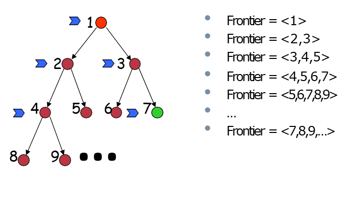
Breadth-First Search (BFS) is a fundamental uninformed search strategy that explores the search tree level by level. It always expands the shallowest unexpanded node in the frontier.

The process is systematic and exhaustive:

Expand the root node (depth 0).

Expand all nodes at depth 1.

Expand all nodes at depth 2.

And so on, until a goal is found.

This ensures that if there are multiple solutions, BFS will first find the one at the shallowest depth. BFS is naturally implemented using a First-In, First-Out (FIFO) queue for the frontier.

The root node is initially placed in the queue.
When a node is expanded, its children (successors) are generated and added to the back of the queue.
The next node to be expanded is always taken from the front of the queue.

This mechanism guarantees that all nodes at depth are expanded before any node at depth .

Algorithm

The following pseudocode describes an efficient implementation of BFS that uses an early goal test and a reached set to avoid redundant paths.

function BREADTH-FIRST-SEARCH(problem) returns a solution node or failure
    node ← NODE(problem.INITIAL)
    if problem.IS-GOAL(node.STATE) then return node
    
    frontier ← a FIFO queue, with node as an element
    reached ← {problem.INITIAL}
    
    while not IS-EMPTY(frontier) do
        node ← POP(frontier)
        for each child in EXPAND(problem, node) do
            s ← child.STATE
            
            if problem.IS-GOAL(s) then return child
            
            if s is not in reached then
                add s to reached
                add child to frontier
    return failure

A key implementation detail is when the goal test is applied.

Late Goal Test: The goal test is applied to a node after it is selected (popped) from the frontier. This is the standard approach for many search algorithms.

def breadth_first_search(problem): 
	node = Node(problem.initial)
	frontier = FIFOQueue([node]) 
	reached = {problem.initial}
 
	while frontier:
		node = frontier.pop()
		
		# Late goal test on the popped node
		if problem.is_goal(node.state): 
			return node
	
		for child in expand(problem, node): 
			s = child.state
			if s not in reached: 
				reached.add(s) 
				frontier.appendleft(child)
	return failure,visited_states

Early Goal Test: The goal test is applied to a node when it is generated, before it is added to the frontier.

def breadth_first_search_early_goal_test(problem):
	node = Node(problem.initial)
	
	if problem.is_goal(problem.initial): 
		return node
	
	frontier = FIFOQueue([node]) 
	reached = {problem.initial} 
	
	while frontier:
		node = frontier.pop()
		for child in expand(problem, node): 
			s = child.state
			
			# Test on the generated node
			if problem.is_goal(s):
				return child
			if s not in reached: 
				reached.add(s) 
				frontier.appendleft(child)
	return failure

For BFS, an early goal test is a valid and more efficient optimization. Because BFS explores level by level, the first time it generates a path to any given state, that path is guaranteed to be the shallowest one possible. Therefore, we can never find a “better” (i.e., shallower) path to that state later on, making it safe to check for the goal upon generation.

Breadth-first search can be viewed as a special case of best-first search algorithm, where the evaluation function is simply the depth of the node—the number of actions taken to reach it. While this generalization is conceptually useful, the native implementation of breadth-first search is more efficient in practice. Using a first-in-first-out (FIFO) queue for the frontier is faster than maintaining a priority queue, which is required for best-first search. Additionally, the reached set in breadth-first search can be a simple set of states, rather than a mapping from states to nodes, because the first path to any state is guaranteed to be the shortest.

As a result, breadth-first search can safely perform an early goal test, checking whether a node is a solution as soon as it is generated, rather than waiting until the node is selected for expansion as in best-first search. This optimization improves both the efficiency and clarity of the algorithm.

Example: BFS for the 8-Queens Puzzle
Breadth-First Search (BFS) can be applied to the 8-Queens puzzle by treating each board configuration as a state. The search starts with an empty board and generates successors by placing a queen in each valid position in the next row, ensuring no two queens attack each other.

Initial State: Empty board (no queens placed).

Actions: Place a queen in any column of the next row where it is not attacked by existing queens.

Goal Test: 8 queens placed on the board, none attacking each other.

BFS explores all possible placements row by row, guaranteeing that the first complete solution found will use the minimum number of moves (8 placements). Because BFS expands all partial solutions at a given depth before moving deeper, it systematically finds all valid arrangements.
def bfs_8_queens():
	frontier = FIFOQueue([empty_board])
	while frontier:
		board = frontier.pop()
		if is_goal(board):
			return board
		for next_board in generate_successors(board):
			frontier.appendleft(next_board)
	return failure
BFS is not the most memory-efficient approach for the 8-Queens puzzle, but it guarantees finding a solution if one exists.

Property	Evaluation	Note
Completeness	Yes	BFS is complete, provided the branching factor is finite. It is a systematic search that is guaranteed to explore every reachable node and will eventually find the shallowest goal.
Optimality	Yes, if all step costs are identical.	Because BFS finds the shallowest solution, and if all steps have the same cost, the shallowest solution is also the cheapest one. However, if costs vary, BFS is not optimal, as a deeper solution might have a lower total cost.
Time Complexity		In the worst case, BFS must generate all nodes up to depth . The total number of nodes generated is , which is dominated by the last term, resulting in a time complexity of .
Space Complexity		The major drawback of BFS is its memory requirement. In the worst case, the frontier must hold all nodes at depth simultaneously. This exponential space complexity often makes BFS impractical for large problems. For a problem with and , storing the frontier could require 10 terabytes of memory, which is a much more significant constraint than the execution time.

Uniform-Cost Search (UCS)

When actions have different costs, BFS is no longer optimal. Uniform-Cost Search (UCS) addresses this by generalizing BFS to find the cheapest path, regardless of the number of steps. Instead of expanding the shallowest node, UCS always expands the unexpanded node in the frontier with the lowest path cost () from the root.

While BFS explores in waves of uniform depth, UCS explores in waves of uniform path cost. It does not necessarily choose the shallowest node, as a path with more steps could have a lower total cost.

UCS is an instance of a best-first search algorithm. It is implemented using a priority queue for the frontier, ordered by increasing path cost . Because a shorter path to a previously seen state might be discovered later, UCS requires a late goal test. The goal test must be applied when a node is selected for expansion, not when it is generated. This ensures that the first time a goal is selected, it is guaranteed to have been reached via the lowest-cost path.

The algorithm can be expressed as a call to a general BEST-FIRST-SEARCH algorithm where the evaluation function is simply the path cost.

function UNIFORM-COST-SEARCH(problem) returns a solution node, or failure
    return BEST-FIRST-SEARCH(problem, PATH-COST)

Property	Evaluation	Note
Completeness	Yes	UCS is complete, provided the branching factor is finite and all step costs are greater than some small positive constant . This prevents the algorithm from getting stuck in infinite loops of zero-cost actions.
Optimality	Yes	Because UCS always expands the node with the lowest path cost, the first goal node it selects for expansion is guaranteed to be at the end of an optimal path.
Time Complexity		The complexity depends not on the depth , but on the cost of the optimal solution, , and the minimum action cost, . This can be much larger than if there are many cheap actions that lead away from the goal, as UCS may explore a large tree of low-cost but suboptimal paths.
Space Complexity		Similar to its time complexity, the space complexity of UCS is also exponential in the ratio of the optimal solution cost to the minimum step cost.

When all action costs are equal (e.g., 1), then and . The complexity becomes , and UCS effectively behaves identically to Breadth-First Search.

def uniform_cost_search(problem):
	node = Node(problem.initial)
	if problem.is_goal(node.state): 
		return node
	
	frontier = PriorityQueue(min, 'path_cost') 
	frontier.append(node) 
	reached = {problem.initial: node} 
	
	while frontier:
		node = frontier.pop()
		
		# Late goal test on the popped node
		if problem.is_goal(node.state): 
			return node
		
		for child in expand(problem, node): 
			s = child.state
			if s not in reached or child.path_cost < reached[s].path_cost: 
				reached[s] = child 
				frontier.append(child)
	return failure

Depth-First Search (DFS)

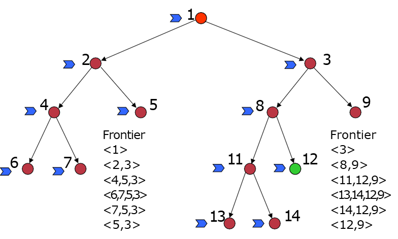
In contrast to the level-by-level exploration of BFS, Depth-First Search (DFS) explores as deeply as possible along one path before backtracking.

The strategy of DFS is to always expand the deepest unexpanded node in the frontier.

Algorithm

It selects the root node and generates one of its successors.

It then immediately expands that successor, generating one of its successors.

This process continues, pushing deeper and deeper into the search tree.

When it reaches a node with no successors (a leaf node) or a previously defined depth limit, it backtracks to the next deepest unexpanded node and explores another path.

This “dive-deep, then backtrack” behavior gives the algorithm its name.

def is_cycle(node, k=30):
	''' Does this node form a cycle of length k or less? ''' 
	def find_cycle(ancestor, k):
		return (ancestor is not None and 
				k > 0 and 
				(ancestor.state == node.state or 
					find_cycle(ancestor.parent, k - 1)))
	
	return find_cycle(node.parent, k)
	
def depth_first_recursive_search(problem, node=None): 
    if node is None:
        node = Node(problem.initial)
    
    if problem.is_goal(node.state):
        return node
    elif is_cycle(node):
        return failure
    else:
        for child in expand(problem, node):
            result = depth_first_recursive_search(problem, child)
            if result:
                return result
        return failure
 
''' Iterative version of the DFS algorithm
def depth_first_search_iterative(problem):
    "Search deepest nodes in the search tree first."
    frontier = LIFOQueue([Node(problem.initial)])
    result = failure
    while frontier:
        node = frontier.pop()
        if problem.is_goal(node.state):
            return node
        elif not is_cycle(node):
            for child in expand(problem, node):
                frontier.append(child)
    return result
'''

DFS is naturally implemented using a Last-In, First-Out (LIFO) queue, also known as a stack, for the frontier.

The root node is initially placed on the stack.
When a node is expanded, its children are generated and added to the front of the stack.
The next node to be expanded is always taken from the front of the stack, which is the most recently generated node.

Unlike BFS and UCS, DFS is often implemented as a tree-like search that does not maintain a reached set of previously visited states. This choice significantly impacts its properties, particularly its memory usage and completeness.

Property	Evaluation	Note
Completeness	No.	In its pure form, DFS is not complete. If the state space contains cycles or infinite paths, DFS can get stuck in an infinite loop, never finding a solution even if one exists. For finite, acyclic state spaces (i.e., true trees), it is complete.
Optimality	No.	DFS returns the first solution it finds. This solution may be located very deep in the tree and is not guaranteed to be the shallowest or least-cost solution.
Time Complexity		Where is the maximum depth of the search tree. In the worst case, DFS may explore the entire tree, which could be much deeper than the shallowest solution (i.e., ). If the tree is infinite, this complexity is also infinite.
Space Complexity		This is the primary advantage of DFS. Because it only needs to store a single path from the root to the current node, along with the unexpanded siblings at each node on that path, its memory requirement is linear with respect to the maximum depth. For problems that would require terabytes of memory with BFS, DFS might only need kilobytes, making it the only feasible option for many large-scale problems.

DFS for State-Finding Problems (e.g., 8-Queens)

For many problems, the path to the goal is the solution (e.g., finding a driving route). However, for problems like the 8-Queens puzzle, the goal is not to find a sequence of actions, but rather a state that satisfies certain conditions (a board with 8 non-attacking queens). In these cases, the goal state itself is the solution, and the path taken to find it is irrelevant. DFS is well-suited for such problems, especially when combined with memory-saving variants like backtracking search.

Dealing with Infinite Paths: DLS and IDS

The primary drawback of DFS is its incompleteness in the face of infinite paths.

This can be resolved by introducing a depth limit.

Depth-Limited Search (DLS)

Depth-Limited Search (DLS) is a simple modification of DFS that imposes a predetermined depth limit, . Any node at depth is treated as if it has no successors.

function DEPTH-LIMITED-SEARCH(problem, l) returns a node or failure or cutoff 
	frontier ← LIFO queue (stack) with NODE(problem.INITIAL) as an element 
	result ← failure 
	
	while not IS-EMPTY(frontier) do 
		node ← POP(frontier) 
		
		if problem.IS-GOAL(node.STATE) then return node 
		
		if DEPTH(node) > l then 
			result ← cutoff 
		else if not IS-CYCLE(node) do 
			for each child in EXPAND(problem, node) do 
				add child to frontier 
	return result

Completeness: DLS is complete if the shallowest solution depth is less than or equal to the limit (). However, if , it will fail to find a solution, making it incomplete in the general case.
Complexity: Its time complexity is and space complexity is .

The main issue is choosing an appropriate value for . If is too small, no solution will be found. If it's too large, it can be inefficient.

def depth_limited_search(problem, limit=40):
	''' Search deepest nodes in the search tree first. ''' 
	frontier = LIFOQueue([Node(problem.initial)]) 
	result = failure
	
	while frontier:
		node = frontier.pop()
		if problem.is_goal(node.state): 
			return node
		''' Limitation '''
		elif len(node) >= limit:
			result = cutoff 
		elif not is_cycle(node):
			for child in expand(problem, node):
				frontier.append(child) 
	return result

Iterative Deepening Search (IDS)

Iterative Deepening Search (IDS) elegantly solves the problem of choosing by trying all possible depth limits in increasing order. It combines the strengths of both BFS and DFS.

Algorithm

The IDS algorithm performs a series of DLS searches:

Run DLS with .
If no solution is found, run DLS with .
If no solution is found, run DLS with .
…and so on, until a solution is found.

function ITERATIVE-DEEPENING-SEARCH(problem) returns a solution node or failure 
	for depth = 0 to ∞ do 
		result ← DEPTH-LIMITED-SEARCH(problem,depth) 
		if result ≠ cutoff then 
			return result

Python Implementation

def iterative_deepening_search(problem):
	''' Do depth-limited search with increasing depth limits. ''' 
	for limit in range(1, sys.maxsize):
		result = depth_limited_search(problem, limit)
		if result != cutoff: 
			return result

While it seems wasteful to regenerate the upper levels of the tree in each iteration, the overhead is surprisingly small. In a search tree, the vast majority of nodes are at the lowest level.

For example, in a tree with and , IDS generates only about more nodes than a single BFS run.

Property	Evaluation	Note
Completeness	Yes	Like BFS, it is guaranteed to find a solution if one exists.
Optimality	Yes, if all step costs are identical	It will find the shallowest solution, which is the optimal one in this case.
Time Complexity		Asymptotically the same as BFS.
Space Complexity		The same as DFS, because at any point it is performing a depth-first search within a given limit.

Iterative deepening is the preferred uninformed search method when the search space is large and the depth of the solution is not known. It combines the guaranteed completeness and optimality (for uniform costs) of BFS with the modest memory requirements of DFS.

Bidirectional Search

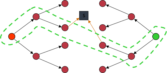
An alternative approach is to search from both ends at once. Bidirectional search runs two simultaneous searches: one forward from the initial state and one backward from the goal state. The search stops when a node from one search frontier is found in the reached set of the other search.

The motivation is that searching two smaller trees of depth is far more efficient than searching one large tree of depth . The total number of nodes generated is approximately , which is significantly less than the of standard BFS or IDS.

Requirements: To search backward, we must have a well-defined goal state (or a small set of them) and be able to compute the predecessors of a state.
Complexity: Time and space complexity are both .

Polimi CS - Notes

Explorer

2.2 - Uninformed Search Strategies

Table of Contents

Tree Search vs. Graph Search

Evaluation of Search Strategies

Breadth-First Search (BFS)

Uniform-Cost Search (UCS)

Depth-First Search (DFS)

Dealing with Infinite Paths: DLS and IDS

Depth-Limited Search (DLS)

Iterative Deepening Search (IDS)

Bidirectional Search

Backlinks

Graph View

Table of Contents