2.3 - Informed Search Strategies

---

Uninformed search strategies, such as Breadth-First or Depth-First Search, are powerful but brute-force. They systematically explore the state space without any knowledge of which states might be closer to a solution. This can be incredibly inefficient for large problems.

Informed search strategies, also known as heuristic search, fundamentally change this approach by incorporating problem-specific knowledge. This knowledge is used to guide the search toward more promising regions of the state space, often finding a solution more quickly and with less computational effort.

The core components of an informed search strategy are:

• Heuristic Function : This function estimates the cost of the cheapest path from the state at node to a goal state. The key word here is estimate. If we knew the actual cost, the problem would already be solved. The heuristic provides an educated guess to guide the search.
• Evaluation Function : This function is used to rank the nodes in the frontier (the set of discovered but not yet expanded nodes). The search algorithm will always choose to expand the node with the best (conventionally, the lowest) value.
• Priority Queue: To efficiently manage the selection process, the frontier is implemented as a priority queue, ordered by the values of the nodes. This ensures that the most “promising” node is always expanded next.

Summary

Criterion	Completeness	Optimality	Time Complexity	Space Complexity
Greedy Best-First Search	No (unless graph search on finite space)	No
A* Search	Yes (finite , positive costs)	Yes (admissible/consistent )
Weighted A* Search	Yes	No (bounded by )
Iterative Deepening A*	Yes	Yes (admissible )	(may be higher due to re-expansion)
Uniform-Cost Search	Yes	Yes

Greedy Best-First Search

Greedy Best-First Search is the simplest form of informed search. It attempts to expand the node that is believed to be closest to the goal, based solely on the heuristic function. It is “greedy” because it makes the locally optimal choice at each step, hoping it will lead to a globally optimal solution.

The evaluation function for Greedy Best-First Search is simply:

This means the algorithm will always expand the node with the lowest estimated cost to reach the goal, regardless of the cost it took to get to that node.

Greedy best-first tree Search python code (it still checks for cycles but has no reached table)

def best_first_tree_search(problem, f):
	'''A version of best_first_search without the reached table.'''
	frontier = PriorityQueue([Node(problem.initial)], key=f) 
	while frontier:
		node = frontier.pop()
		if problem.is_goal(node.state): 
			return node
		for child in expand(problem, node):
			if not is_cycle(child): 
				frontier.add(child)
	return failure

Best-first Greedy Search python code (with reached table)

def best_first_search(problem, f):
	'''Search nodes with minimum f(node) value first.''' 
	node = Node(problem.initial)
	frontier = PriorityQueue([node], key=f)
	reached = {problem.initial: node} 
	
	while frontier:
		node = frontier.pop()
		if problem.is_goal(node.state): 
			return node
		for child in expand(problem, node):
			s = child.state
			if s not in reached or child.path_cost < reached[s].path_cost:
				reached[s] = child
				frontier.add(child) 
	return failure

Heuristics for the 8-Puzzle

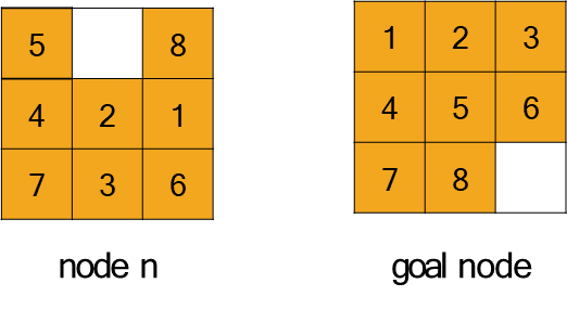
Let’s consider the 8-puzzle problem to understand how heuristics work. Our goal is to transform a given starting configuration into a target goal configuration. Two common heuristics are:

1. : Number of Misplaced Tiles. This heuristic simply counts how many tiles (not including the blank space) are not in their correct goal position. This is based on a relaxed problem where we can move any tile to its correct position in a single step, ignoring the constraint that tiles must slide into an adjacent empty space.
2. : Sum of Manhattan Distances. This heuristic is more sophisticated: for each tile, it calculates the number of horizontal and vertical steps required to move it from its current position to its goal position. The sum of these distances for all tiles is the heuristic value. This is also a relaxed problem, where each tile can move freely without interfering with others.

• : Tiles 5, 8, 2, 1, 3, and 6 are misplaced. Tiles 4 and 7 are in the correct position. Therefore, .
• :

  • Tile 5: 1 step right, 1 step down →

  • Tile 8: 2 steps down, 1 step left →

  • Tile 4: 0 steps →

  • And so on for all tiles… The total sum is .

Notice that provides a more accurate estimate of the remaining cost than . An algorithm using is considered more "informed" than one using .

Both and are constructed by solving “relaxed versions” of the original problem, each removing certain constraints to make the problem easier. When comparing two consistent heuristic functions, and , if for every node :

then is said to dominate . This means that provides equal or higher estimates of the remaining cost for every state, without ever overestimating the true cost (since both are admissible and consistent).

If dominates , every node expanded by the GBFS algorithm using will also be expanded when using , but not necessarily vice versa. In other words, GBFS guided by a more dominant heuristic will generally expand fewer nodes, making the search more efficient.

In the context of the 8-puzzle: (Manhattan distance) dominates (misplaced tiles), since for any configuration, .

When one heuristic dominates another, we say it is more accurate or more informed. Using a more informed heuristic leads to faster solutions and reduced computational effort in heuristic search algorithms.

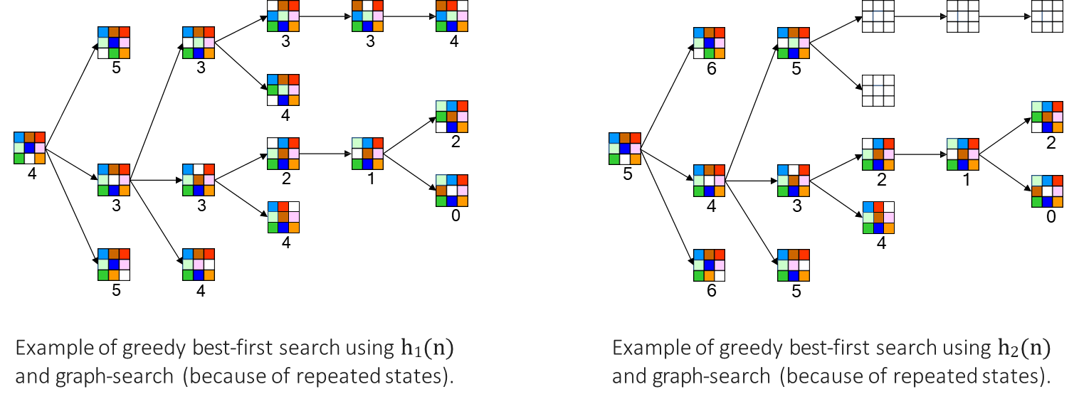
Example

Let’s revisit the 8-puzzle problem and visualize the search process as a tree, where each node represents a configuration and is annotated with its heuristic value.

• Using (Misplaced Tiles): Starting from the initial configuration, we consider all possible moves for the blank space. At each step, we select the child node with the lowest value, moving towards configurations with fewer misplaced tiles. This process continues until we reach the goal configuration, where .

• Using (Manhattan Distance): Similarly, we begin with the initial configuration, which typically has a higher value. At each step, we choose the move that leads to the configuration with the lowest value, prioritizing states that are closer to the goal in terms of total tile movements.

Both heuristics guide the search towards the goal, but their estimates differ. For example, might estimate that four moves are needed, while estimates five moves. These are only approximations—the actual number of moves required may vary. However, a more accurate heuristic (like ) generally leads to a more efficient search, expanding fewer nodes and reaching the solution faster.

Limitations of Greedy Search

While often fast, the greedy approach has significant drawbacks:

1. Incompleteness: If the search space contains loops, a greedy algorithm can get stuck in an infinite loop, never finding a solution even if one exists. Using a reached table (graph search) can solve this for finite state spaces.
2. Suboptimality: The algorithm is not optimal. It can be drawn towards a dead-end or a path that seems promising locally but is globally very costly. This is often called the “local minima problem.”

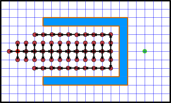
Example

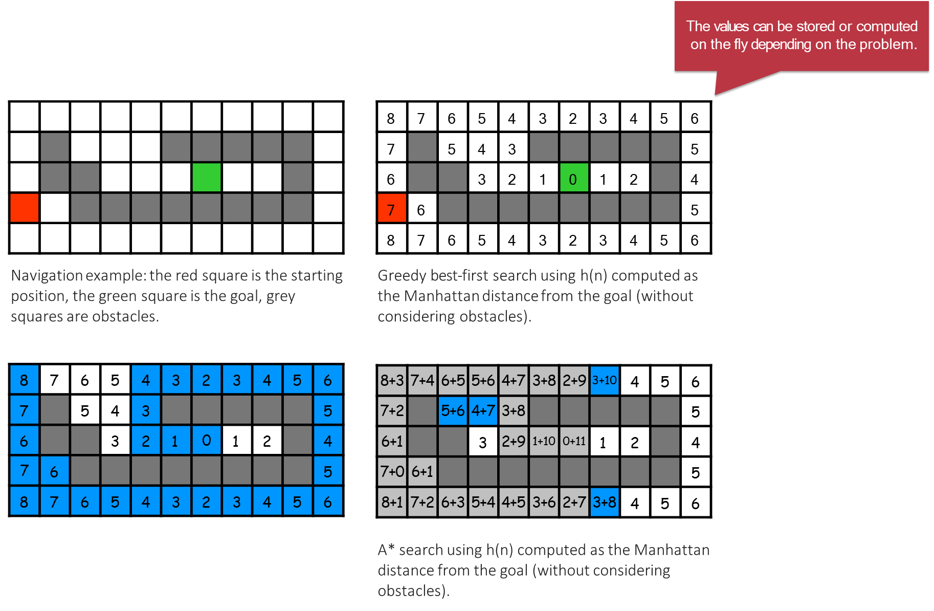
An agent using a straight-line distance heuristic will move directly towards the goal. However, if there is a C-shaped obstacle, it will get stuck at the bottom of the “C”.

To escape, it must temporarily move away from the goal, which increases the heuristic value. A greedy algorithm will refuse to do this, becoming trapped.

3. Complexity: The worst-case time and space complexity is , where is the branching factor and is the maximum depth of the search space.

A* Search

Search is the most widely-known and effective informed search algorithm. It improves upon Greedy Best-First search by considering both the cost to reach a node and the estimated cost to get from that node to the goal.

The evaluation function for Search is:

where:

• : The actual cost of the path from the start node to node . This is what we know for sure.
• : The estimated cost of the cheapest path from node to the goal. This is what we are guessing.

Therefore, represents the estimated cost of the cheapest solution that passes through node .

Search python code (with reached table).

def g(n): 
	return n.path_cost
 
def astar_search(problem, h=None):
	'''Search nodes with minimum f(n) = g(n) + h(n).''' 
	h = h or problem.h
	return best_first_search(problem, f=lambda n: g(n) + h(n))
 

Note that the algorithm is implemented using the Best-First Search algorithm: this is because is a specific instance of Best-First Search where the evaluation function is defined as .

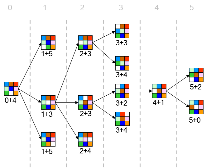
Example

Let’s revisit the 8-puzzle problem using a tree representation, this time applying the algorithm to reach the goal configuration. In this tree, each node (configuration) is annotated with two values:

• The number of steps taken so far (), representing the distance from the initial configuration.
• The number of misplaced tiles (), serving as our heuristic estimate.

At each step, the algorithm selects the node with the lowest sum , which combines the actual cost incurred and the estimated cost to reach the goal. The search proceeds by expanding nodes in order of increasing values. If a newly generated configuration has a higher than the current minimum, it is not expanded in this iteration.

This process ensures that always expands the most promising configurations first, balancing progress toward the goal with the cost already incurred. The search terminates when the goal configuration is reached (), and the path found is guaranteed to be optimal if the heuristic is admissible.

By incorporating , avoids the primary pitfall of Greedy search. It balances the need to make progress towards the goal () with the need to avoid excessively long paths ().

Example

Let’s revisit the navigation example where Greedy search gets stuck.

• Greedy Search only sees . It moves into the C-shaped obstacle because is decreasing. Once at the bottom, any move away from the goal increases , so it gets stuck.
• Search sees . As it moves deeper into the obstacle, the path cost steadily increases. Eventually, the value for nodes inside the obstacle will become higher than the value for nodes on an alternate, longer path around the obstacle. will then correctly choose to expand the node on the path around the obstacle, leading it away from the suboptimal path and towards the correct solution.

By using both the cost so far and the estimate of the cost of reaching the goal , can lead the agent away from suboptimal paths.

Completeness

Search is complete, meaning it will always find a solution if one exists, under two conditions:

1. The search space has a finite branching factor.
2. All action costs are positive (greater than some small constant ).

The reasoning is straightforward: if a solution exists, it has a finite cost, let’s call it . As the search algorithm explores paths, the component (path cost) will continuously increase for every step taken. Any path that wanders off infinitely will eventually have a value greater than . Since always expands the node with the lowest , it will not expand these infinitely long paths forever and is guaranteed to eventually find the solution path.

While is complete, its optimality (finding the least-cost solution) is not guaranteed by default. For to be optimal, the heuristic function must satisfy certain properties, primarily admissibility and consistency.

Admissible Heuristics

While search is complete, its most celebrated property is its ability to find the optimal (least-cost) solution. However, this guarantee is not automatic; it depends entirely on the quality of the heuristic function . The key property required for optimality is admissibility.

Definition

An admissible heuristic is one that is fundamentally optimistic: it never overestimates the true cost to reach the goal.

Formally, a heuristic function is admissible if, for every node :

where is the true cost of the optimal path from node to a goal node. A natural consequence of this is that for any goal node , must be 0.

A common and effective way to design an admissible heuristic is to consider a relaxed version of the problem. Because the relaxed problem has fewer constraints, the optimal solution cost in the relaxed problem is guaranteed to be less than or equal to the optimal solution cost in the original, more constrained problem. This cost becomes our admissible heuristic.

Admissible heuristic function for the 8-puzzle

• (Misplaced Tiles): This heuristic is the solution cost to a relaxed problem where a tile can be moved from any square to any other square in a single step. Since each misplaced tile must be moved at least once in the real problem, never overestimates the remaining moves. Thus, it is admissible.
• (Manhattan Distance): This is the solution cost to a relaxed problem where a tile can slide to any adjacent square, even if occupied by another tile. Since this ignores the interference of other tiles, it represents a shorter or equal path than what is achievable in the real puzzle. Thus, is also admissible.

Admissible heuristic function for the navigation problem

• Euclidean Distance: The straight-line distance is the solution cost to a relaxed problem where the agent can move in a straight line to the destination, ignoring obstacles and road networks. This is the shortest possible path, so it is admissible.
• Manhattan Distance: This is the optimal cost if the agent can only move horizontally and vertically. If diagonal moves are also allowed in the original problem, the Manhattan distance might overestimate the true cost. For example, to move one unit right and one unit down, the Manhattan distance is . The true diagonal cost is . Since , the Manhattan distance is not admissible if diagonal movement is allowed.

Optimality of A* with an Admissible Heuristic (Tree Search)

With an admissible heuristic, used with a tree-search algorithm is guaranteed to return an optimal solution.

Optimality Theorem:

If is an admissible heuristic, then tree search is optimal.

Proof by Contradiction (Intuition):

Let be the cost of the optimal solution path. Assume terminates by returning a suboptimal goal node with a path cost . Because , the evaluation function for this suboptimal solution is .

At some point before was chosen for expansion, there must have been at least one node in the frontier that was on the true optimal path to the actual optimal goal . For this node , its evaluation function is .

Because is admissible, we know . Therefore, . The term is, by definition, the cost of the true optimal path, which is .

This gives us . Since we know , it follows that .

This creates a contradiction: could not have selected for expansion, because the more promising node (with a lower -value) was still in the frontier. Therefore, will never select a suboptimal goal, and the algorithm must be optimal.

Consistent Heuristics and Graph Search

While admissibility guarantees optimality for tree search, graph search (which discards already visited states) requires a stricter condition known as consistency.

Definition

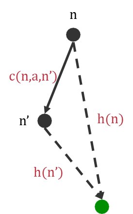
A heuristic is consistent (or monotonic) if, for every node and every successor generated by an action , the estimated cost from is no greater than the step cost to plus the estimated cost from .

This is a form of the triangle inequality:

Consistency is a stronger property than admissibility.

• Every consistent heuristic is also admissible. Thus, with a consistent heuristic, tree search is cost-optimal (both using tree-search and graph-search).
• Not every admissible heuristic is consistent.

In addition, with a consistent heuristic, the first time we reach a state, it will be on an optimal path to that state. This is because the -values along any path are non-decreasing, ensuring that once a node is expanded, we have found the least-cost path to it. Thus, we never have to re-add a state to the frontier and never change an entry in the reached table.

When is an heuristic function not consistent?

Consider an heuristic function for which the estimated cost to the goal node from is , the cost of moving from to its successor is , and the estimated cost to the goal node from is .

In this case the triangular inequality does not hold since

so the heuristic is not consistent. However, it is still admissible since does not overestimate the true cost to reach the goal from .

Example

Considering the navigation problem and considering the following heuristic functions:

• Euclidean Distance: . is consistent because the straight-line distance between two points is always less than or equal to the distance of any path connecting those points, satisfying the triangle inequality.
• Manhattan Distance: . is also consistent if we move only in horizontal and vertical directions, while it is not consistent if diagonal moves are allowed.

The primary benefit of a consistent heuristic is that it guarantees that the -values of nodes along any path will be non-decreasing.

From the consistency property, we can rearrange to get . Substituting this into the equation for does not lead to a simple .

This means that as expands nodes, it does so in concentric contours of increasing -cost. A critical consequence of this is:

When with a consistent heuristic selects a node for expansion, it has already found the optimal (least-cost) path to .

This simplifies graph search immensely. If we have already visited a state, we never need to consider a new path to it, because the first path found is guaranteed to be the best.

Optimality of with an Admissible Heuristic (Graph Search)

Optimality Theorem (Graph Search):

If is a consistent heuristic, then graph search is optimal.

Proof

Consider as a successor of node . By the definition of and the consistency property, we have:

This shows that search expands nodes in non-decreasing order of . When selects a node from the frontier, the path to that state is guaranteed to be optimal. Therefore, when selects the first goal node from the frontier, it is the optimal solution.

If the heuristic is admissible but not consistent, graph search may return a suboptimal solution.

Example

1. We have a starting node and a goal . is admissible.
2. From , we can reach state via two paths:
   • Path 1: , total cost = . Let’s say . .
   • Path 2: , total cost = . Let’s say . .
3. The heuristic is inconsistent because might be high, while is very low, violating the triangle inequality.
4. Suppose the search algorithm first explores the long path and finds state with cost . It adds to the reached set.
5. Later, it explores the shorter path and finds state again, this time with cost .
6. Because this is graph search, it checks the reached set, sees that state has already been found, and discards this new, better path.
7. The algorithm proceeds with the suboptimal path to , potentially leading to a suboptimal final solution.

In contrast, tree search would keep both nodes representing the state (one for each path) in the frontier and would correctly expand the one on the optimal path.

Some implementations deal with the issues of inconsistent heuristics by entering a state into the frontier only once. If a better path to the state is found, all the successors of the state are updated. This requires nodes to have both child and parent pointers.

Further Properties and Practical Considerations

Optimal Efficiency of A*

Beyond being complete and optimal, is also optimally efficient. This means that for a given heuristic, no other optimal algorithm is guaranteed to expand fewer nodes than . expands all nodes with , some nodes with , and no nodes with . It is the most efficient search possible under these conditions because it must expand every node with to prove that no better path exists.

The Trivial Heuristic: h₀(n) = 0

What if we have no domain knowledge to create a good heuristic? We can use the simplest possible admissible and consistent heuristic:

This heuristic is trivially admissible () and consistent (). Let’s see what happens to ‘s evaluation function:

The algorithm simplifies to expanding the node with the lowest path cost . This is precisely the definition of Uniform-Cost Search. Therefore, Uniform-Cost Search can be seen as a special case of search where the heuristic provides no information.

Satisficing Solutions

expands a large number of nodes to guarantee optimality. In many real-world scenarios (like video games or real-time robotics), finding a perfect solution slowly is less useful than finding a “good enough” solution quickly.

These “good enough,” suboptimal solutions are called satisficing solutions. We may be willing to trade the guarantee of optimality for a significant reduction in search time and memory usage. This leads to variations of that intentionally use inadmissible heuristics to speed up the search, a concept explored in the next section with Weighted .

Memory-Bounded and Advanced Heuristic Search

While is optimally efficient, its primary drawback is its memory usage. For large problems, the number of nodes stored in the frontier and the reached set can become prohibitively large, exhausting available memory. This section explores algorithms designed to address these memory limitations and find solutions under constraints.

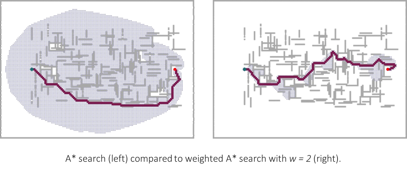
Weighted A* Search

One way to reduce the number of expanded nodes is to make the search more “greedy” without completely abandoning the path cost . This is the core idea behind Weighted Search.

Weighted modifies the standard evaluation function by introducing a weight on the heuristic component:

• When , it is standard search.
• When is very large, the search becomes similar to Greedy Best-First Search.
• When , the heuristic’s influence is amplified. This makes the search more aggressive, focusing more on nodes that appear close to the goal.

This approach uses an inadmissible heuristic ( can overestimate the true cost if was admissible). The direct consequence is that Weighted is not optimal. However, it comes with a useful bound: the cost of the solution found will be no more than times the cost of the optimal solution.

Advantages:

• Faster: By focusing the search more narrowly towards the goal, Weighted typically expands far fewer nodes than standard .
• Bounded Suboptimality: It provides a guarantee on how far from optimal the solution can be.

Iterative Deepening A* (IDA*)

Iterative Deepening () is a direct answer to the memory problem of . It combines the idea of iterative deepening search with the heuristic guidance of . Instead of a depth limit, uses an -cost limit (referred to as a “cutoff”).

The algorithm works in iterations:

1. Initialize: The initial cutoff is set to the -cost of the start node, f(start_node) = h(start_node).
2. Iterate:
   1. Perform a depth-first search from the start node. Prune any path as soon as its -cost exceeds the current cutoff.
   2. If a goal node is found, the algorithm terminates, returning the solution. Since paths are explored in increasing order of -cost, the first solution found is guaranteed to be optimal if is admissible.
   3. If the entire search space is explored without finding a solution within the cutoff, the iteration ends. The new cutoff is set to the smallest -cost of any node that was generated but pruned during the last iteration.
3. Repeat: Go back to step 2 with the new, higher cutoff.

Example

• Iteration 1: cutoff is set to f(start) = 0+4 = 4. The DFS explores, but any node where is immediately pruned. No solution is found. The smallest -cost of a pruned node was 5.
• Iteration 2: cutoff is set to 5. The DFS is run again. It re-explores the previous nodes and can now go deeper, expanding nodes with -costs of 5. The algorithm proceeds until it finds a goal or prunes all paths.

Properties of :

• Completeness and Optimality: ID is complete and optimal under the same conditions as (finite branching factor, admissible heuristic).
• Memory Complexity: Its memory requirement is only proportional to the depth of the solution, , because it is fundamentally a depth-first search. This is its greatest advantage.
• Time Complexity: It can be inefficient time-wise. States are repeatedly generated in each iteration. For problems with a large number of unique -cost values, this can be very costly, as each new iteration might only expand one additional node.