5 - Learning to Search and Play

---

Machine Learning Introduction

The central question posed at the outset is fundamental: “How can computer programs learn?” This question moves us away from the traditional paradigm of explicit programming, where a human defines every rule and logic, towards a new paradigm where systems can improve through experience.

A formal and widely accepted definition of machine learning was provided by Tom M. Mitchell in 1997:

"A computer program is said to learn from experience with respect to some class of tasks and performance measure , if its performance at tasks in , as measured by , improves with experience .”

This definition provides a clear framework for any machine learning problem:

• Task (): What is the program supposed to do? (e.g., play a game, classify an image, predict a price).
• Experience (): What data or interactions does the program use to learn? (e.g., a dataset of past games, a collection of labeled images, historical stock market data).
• Performance Measure (): How do we evaluate if the program is getting better? (e.g., percentage of games won, accuracy of classifications, error in price prediction).

Definition

Machine Learning is a subfield of Artificial Intelligence focused on building algorithms that can extract knowledge from experience.

It is crucial to understand that these algorithms do not create knowledge from nothing; they identify and generalize patterns present in the data they are given. The ultimate goal is to build programs capable of making informed, intelligent decisions on new, previously unseen data.

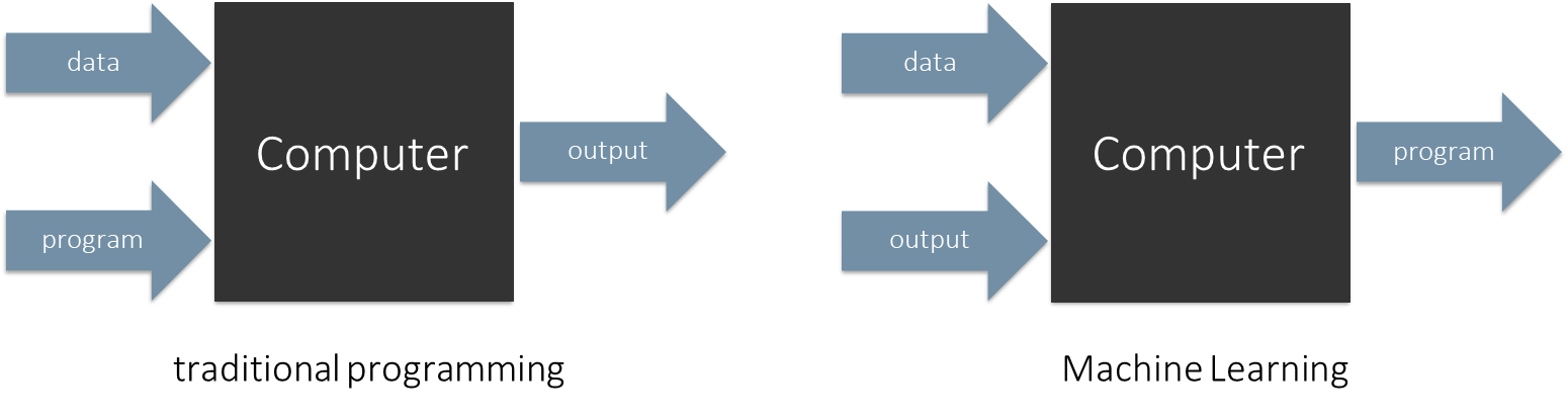
To fully appreciate machine learning, it’s helpful to contrast it with the traditional programming approach.

• Traditional Programming: A programmer takes input data and a set of explicit rules (the program) and feeds them into a computer. The computer processes the data according to these rules and produces an output. The logic is entirely human-defined.

  • Input: Data, Program
  • Process: Computer
  • Output: Output

• Machine Learning: The paradigm is inverted. A developer provides the computer with input data and the corresponding desired outputs (the “experience”). The machine learning algorithm then works backward to determine the rules or patterns that map the inputs to the outputs. This learned model is, in essence, the program.

  • Input: Data, Output (experience, examples)
  • Process: Computer
  • Output: Program (Model)

Given a dataset of experience, , there are three primary ways a program can learn from it.

Paradigm	Description	Key Characteristics
Supervised Learning	The algorithm is given a dataset where each data point is paired with a desired output or “label” . It learns a mapping function from inputs to outputs, with the goal of correctly predicting the output for new, unseen data points.	- Desired output is known (labels, numbers). - Receives direct feedback on its predictions during training. - Used for prediction tasks (e.g., classification, regression).
Unsupervised Learning	The algorithm is given a dataset without any explicit labels. It must discover the underlying structure, patterns, or regularities within the data on its own.	- No desired output to predict. - No feedback about predictions. - Goal is to “find hidden structure” (e.g., clustering, dimensionality reduction).
Reinforcement Learning	The algorithm, or “agent,” learns by interacting with an environment. It performs actions that change the state of the environment and receives rewards or penalties in return. The goal is to learn a sequence of actions (a policy) that maximizes its cumulative long-term reward.	- Involves a decision-making process (actions). - Learns from an immediate reward system. - Focused on long-term expectation, not just immediate gain. - Learns a sequence of actions.

Foundations of Reinforcement Learning (RL)

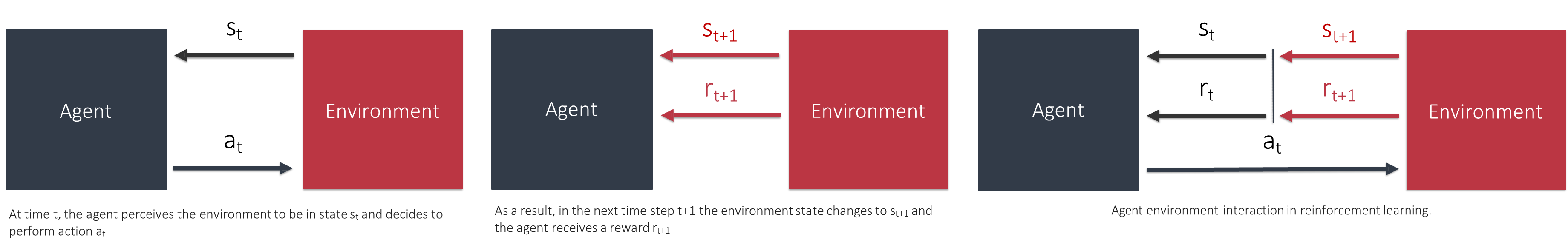
Reinforcement Learning (RL) is a paradigm of learning through trial and error, inspired by behavioral psychology. It is particularly suited for problems that involve making a sequence of decisions over time to achieve a goal. The core of RL is the interaction between an agent and an environment. This interaction unfolds over a sequence of discrete time steps ().

Steps

The cycle proceeds as follows:

1. Observe State: At a given time , the agent observes the current state of the environment, denoted as .
2. Take Action: Based on the state , the agent selects and performs an action, .
3. Receive Feedback: The action affects the environment. As a result, at the next time step , the environment transitions to a new state, , and provides the agent with a numerical reward, .

This loop repeats, generating a trajectory of states, actions, and rewards: .

• Agent: The learner and decision-maker.
• Environment: Everything outside the agent that it interacts with.
• State (): A complete description of the environment at a specific time.
• Action (): A choice made by the agent that influences the environment.
• Reward (): A scalar feedback signal indicating how good the agent’s action was in the short term.

Reinforcement Learning addresses problems of sequential decision making, which have several key characteristics:

• The goal is achieved by taking a sequence of decisions (actions) over time, not just a single decision.
• The best (optimal) actions are context-dependent; the right action to take depends entirely on the current state of the environment and not just on immediate rewards.
• We often do not have examples of correct actions. The agent must discover them for itself through exploration.
• Actions can have long-term consequences. An action that yields a small immediate reward might lead to a much larger reward later, or vice versa.
• The short-term consequences of optimal actions might even seem negative. For example, a chess player might sacrifice a pawn (a short-term loss) to gain a strategic advantage that leads to winning the game (a long-term gain).

The agent’s sole objective is to maximize the total amount of reward it receives over the long run. This fundamental principle is captured by Rich Sutton’s Reward Hypothesis:

"That all of what we mean by goals and purposes can be well thought of as maximization of the expected value of the cumulative sum of a received scalar signal (reward)."

This is a powerful idea: any goal can be framed as maximizing a cumulative reward signal.

This makes the design of the reward function critical. It must adequately represent the learning goal.

Examples of Reward Functions:

• Goal-Reward: Return a reward of when the goal is reached, and otherwise. This is sparse but clearly defines the goal.
• Action-Penalty: Return a reward of for every action taken when the goal is not reached, and once the goal is reached. This encourages the agent to find the goal in the fewest steps possible.

However, this hypothesis also presents challenges, such as how to design reward functions that encourage complex behaviors like risk-sensitivity or diversity.

Core Concepts in Reinforcement Learning

The Value Function

While rewards provide immediate feedback, the agent needs a way to estimate the long-term, cumulative reward. This is the role of value functions. They map states or state-action pairs to an expected future payoff.

There are two primary types of value functions:

1. State-Value Function, : This function estimates the expected total future reward an agent can expect to receive starting from state and following a specific policy thereafter. It answers the question, “How good is it to be in this state?”
2. Action-Value Function, : This function estimates the expected total future reward an agent can expect to receive by taking action in state and following a specific policy thereafter. It answers the question, “How good is it to take this action from this state?” We often write this as .

Example

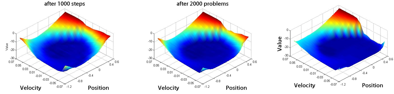
The Mountain Car task is a classic RL problem that illustrates these concepts.

• Task: Drive an underpowered car up a steep hill to reach the goal at the top.
• Challenge: The car’s engine is not strong enough to drive directly up the hill. The agent must learn to build momentum by driving back and forth.
• State (): The car’s position and velocity.
• Actions (): Accelerate left, accelerate right, or do nothing (coast).
• Reward (): for every time step until the goal is reached, and when the goal is reached.

![[Foundation of Artificial Intelligence/img/9 - Learning to Search and Play-1760961791712.png|The image shows a learned state-value function for this task. The lowest values (the deep blue “valley”) are in the center at low velocity, representing states where it is difficult to reach the goal. The highest value (the red peak) is at the goal position. The function correctly captures that high velocity, even when moving away from the goal, is valuable because it helps build momentum.|593x316]]

Value functions adhere to a crucial recursive relationship known as the Bellman Equation. It decomposes the value of a state into the sum of the immediate reward and the discounted value of the next state. This allows us to solve for the value functions iteratively.

The Bellman Expectation Equation for the state-value function is:

The value of the current state is the expected immediate reward plus the discounted () expected value of the next state .

Similarly, for the action-value function :

This can be broken down into two key components: the incoming reward () and the value of the next state ().

The Agent’s Strategy

A policy, denoted by , is the agent’s strategy or behavior. It is a mapping from states to actions, defining what action the agent will take in any given state.

• Deterministic Policy: The policy maps each state to a single, specific action . For example, a policy might be to always select the action with the highest Q-value: . This can be represented simply in a lookup table.
• Stochastic Policy: The policy maps each state to a probability distribution over the available actions. It returns the probability of selecting action in state . For example, in state , the policy might be: .

To maximize its reward, the agent must find a balance between two competing needs:

• Exploitation: Prefer actions that it has tried in the past and found to lead to a high payoff. This means using its current knowledge to get rewards.
• Exploration: Try actions that it has not selected before. This is necessary to discover new, potentially better actions.

This is the exploration-exploitation dilemma. If the agent only exploits, it might get stuck with a suboptimal strategy. If it only explores, it will never capitalize on its knowledge to earn a high reward.

A simple and effective way to manage this trade-off is the ε-Greedy Policy:

• With probability (a high probability, e.g., ), the agent exploits by choosing the action with the highest estimated Q-value.
• With probability (a small probability, e.g., ), the agent explores by choosing a random action.

The Environment: Markov Decision Processes (MDPs)

For Reinforcement Learning methods to be applicable, the environment must satisfy the Markov Property.

The Markov Property

The future is independent of the past, given the present.

This means that the next state and reward depend only on the current state and the current action . The entire history of states and actions before is irrelevant.

An environment that satisfies this property can be formally modeled as a Markov Decision Process (MDP). An MDP is defined by its one-step dynamics, which is a probability distribution . This function specifies the probability of transitioning to state and receiving reward , given that the agent was in state and took action . So, we can write that:

in other words, the probabilities of all possible next states and rewards must sum to 1 for any given state-action pair.

The Payoff

The agent’s goal is to maximize its cumulative reward, also known as the return, . For a finite task, this is simply the sum of all future rewards. However, for a continuing task that could go on forever, this sum could be infinite.

To handle this, we introduce a discount factor, (gamma), where . The discounted return is defined as:

thus, the expected reward to maximize becomes the sum of all future rewards, each multiplied by an exponentially decreasing weight determined by .

The discount factor has two key effects:

1. Mathematical Convenience: It ensures that the sum is finite, as long as rewards are bounded. The sum is guaranteed to be .
2. Behavioral Modeling: It values immediate rewards more than future rewards. A close to 0 makes the agent “myopic” (short-sighted), while a close to 1 makes it “far-sighted.”

The agent’s goal is thus to choose actions that maximize the expected discounted return.

An Algorithm for Learning: Q-Learning

Q-learning is a fundamental RL algorithm used to find the optimal action-value function, . It is an “off-policy” algorithm, meaning it can learn the optimal policy even while following a suboptimal (exploratory) policy like ε-Greedy.

In its simplest form (tabular Q-learning), the algorithm maintains a table of Q-values for every state-action pair. This table is initialized with random values.

Formula

At each time step , after taking action from state and observing the reward and new state , the agent updates its Q-table using the following rule:

• : The old Q-value, or what the agent previously thought the value of this state-action pair was.
• (beta): The learning rate (often denoted by , alpha), a value between 0 and 1 that controls how much the new information overrides the old. If is big (close to 1), the agent heavily weights the new information. If is small (close to 0), it relies more on past knowledge.
• : The incoming reward.
• : The discounted estimate of optimal future value. This is the core of Q-learning. It looks at the next state and finds the maximum possible Q-value for any action that can be taken from there. This represents the best the agent can hope to achieve from .
• : This entire term is the temporal-difference (TD) error. It’s the difference between the new, improved estimate of the Q-value and the old estimate. The agent is learning from this error.

In simpler terms, the update rule is:

Tabular Q-learning is a powerful concept, but it has a severe limitation: it assumes we can create and store a table with an entry for every possible state-action pair.

As seen in the Mountain Car example, even a simple problem with continuous states (position and velocity) has an infinite number of states. In more complex problems like chess or Go, the number of states is astronomically large.

• The real world is complex; the number of possible inputs can be huge.
• Storing an exact table is infeasible for most interesting problems.

This forces us to move from exact representations to approximations. Instead of a table, we can use a function approximator (like a linear function or a neural network) to estimate the Q-values.

However, this introduces a new challenge: Reinforcement learning is now trying to compute an unknown value function while simultaneously trying to approximate it. The approximator works on intermediate, constantly changing estimates, which can lead to instability. Unlike tabular Q-learning, convergence is not guaranteed when using powerful function approximators. This trade-off between scalability and stability is a central theme in modern reinforcement learning.

Informed Search vs. Reinforcement Learning

Having established the foundational concepts of Reinforcement Learning, we now turn to a crucial question: how does this learning-based approach compare to the search algorithms discussed previously? While both can be used to solve problems like navigating a maze, they operate on fundamentally different principles and produce profoundly different kinds of solutions.

The most significant difference lies in the nature of their output.

• Informed Search (e.g., [[Foundation of Artificial Intelligence/2.3 - Informed Search Strategies#a-search|A]]):* Given a complete model of the environment (the map, action costs, and goal location), a search algorithm computes a plan. A plan is a specific sequence of actions to get from a single start state to a goal state. It is an explicit solution path. If the agent deviates from the path or the start position changes, a new search must be performed.
• Reinforcement Learning (e.g., Q-Learning): An RL agent, often starting with no model of the environment, learns a policy. A policy, , is a complete mapping that specifies the best action to take from any given state. It is a universal, reactive strategy, not a fixed path.

To illustrate this, we will examine two case studies.

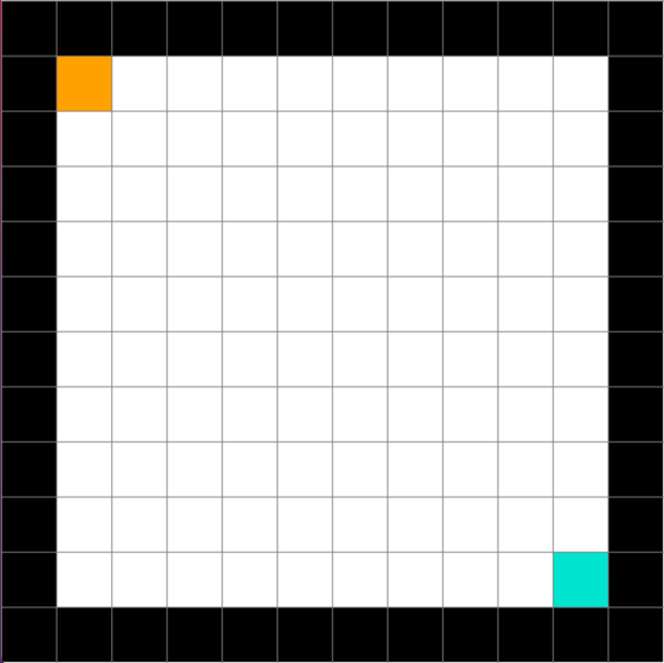
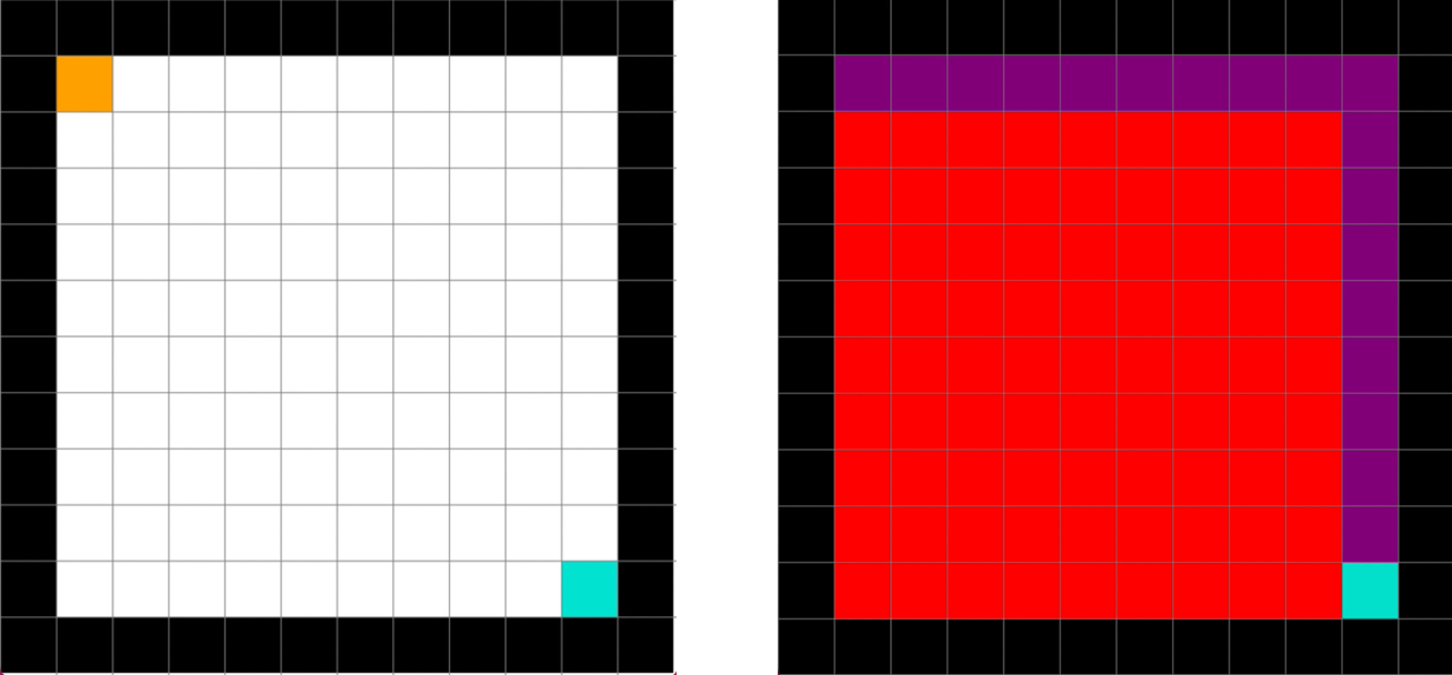
Case Study 1: The Empty Grid World

Consider a simple, empty 10x10 grid environment. The world is bounded by walls. The agent has a single starting position (orange) and a single goal position (blue).

If we apply an informed search algorithm like A* (or a simpler one like breadth-first search, which is sufficient here) to this problem, the algorithm explores the state space systematically from the start position. It keeps track of visited nodes and expands its frontier until it finds the goal.

The result of the search is a single, optimal path from the start to the goal. The visualization below shows the nodes explored by the algorithm (in red - states that are explored by the algorithm - and purple - that represents the solution states) to find this path. The algorithm has solved this specific problem instance.

Now, let’s frame the same problem for a Q-learning agent.

1. Defining the Reward Function: First, we must design a reward function. A simple and effective choice for this type of goal-oriented task is a sparse reward signal:

• Receive a reward of upon reaching the goal state (blue square).
• Receive a reward of for all other transitions.

This setup encourages the agent to reach the goal but does not explicitly tell it how. The agent must discover the path to the reward through exploration.

2. The Learning Process: The agent begins by knowing nothing about the environment. It explores, taking random actions. Initially, it wanders for a long time before accidentally stumbling upon the goal. When it finally does, it receives the +1 reward. Through the Q-learning update rule, this reward signal begins to propagate backward to the state-action pair that led to the goal. Over many episodes (attempts to solve the problem), this value continues to back-propagate through the grid, creating a “gradient” of increasing Q-values that lead toward the goal.

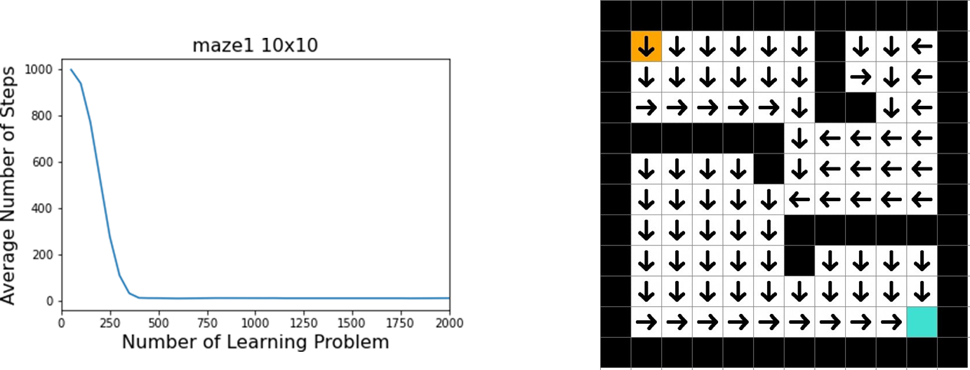
The performance of the agent can be measured by the number of steps it takes to reach the goal in each episode. The graph below shows the average number of steps (smoothed over the last 100 episodes) as the number of learning episodes increases. We observe a classic learning curve:

• Initial Phase (Episodes 0-150): The agent takes a very high number of steps. It is exploring randomly and has not yet reliably learned the path to the reward.

• Learning Phase (Episodes 150-250): There is a dramatic drop in the number of steps. The agent has experienced the reward enough times that the value has propagated significantly, and its policy is quickly improving.

• Convergence Phase (Episodes 250+): The agent consistently solves the problem in a small, optimal number of steps. It has learned an effective policy.

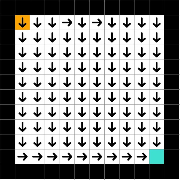
3. The Learned Outcome: A Policy After sufficient training, the agent’s learned knowledge is not a single path but a complete policy. We can visualize this by placing an arrow in each grid cell indicating the best action to take from that state (i.e., the action with the highest Q-value).

This policy is far more robust than the single plan found by the search algorithm. If the agent were dropped into any empty square, it would instantly know the best direction to move to reach the goal.

3. Under the Hood: The Action-Value Function The policy visualization is derived from the learned action-value function, which is stored in the Q-table. The table below shows a portion of the final Q-table. Each row corresponds to a state (a grid cell), and the columns show the learned value for taking each of the four possible actions (Up, Right, Down, Left) from that state.

Example

State	Up	Right	Down	Left
(1, 2)	0.397	0.440	0.440	0.000
(1, 3)	0.418	0.463	0.463	0.000
(1, 4)	0.440	0.488	0.488	0.000
…	…	…	…	…
(2, 1)	0.000	0.440	0.440	0.397
(2, 2)	0.418	0.463	0.463	0.418
(2, 3)	0.440	0.488	0.488	0.440
…	…	…	…	…

For example, from state (2, 3), the best actions are ‘Right’ and ‘Down’ (both with a value of 0.488), which aligns with the policy map pointing towards the goal in the bottom-right corner. The value of 0.000 for action ‘Left’ from state (1, 2) correctly reflects that this action is suboptimal as it moves away from the goal.

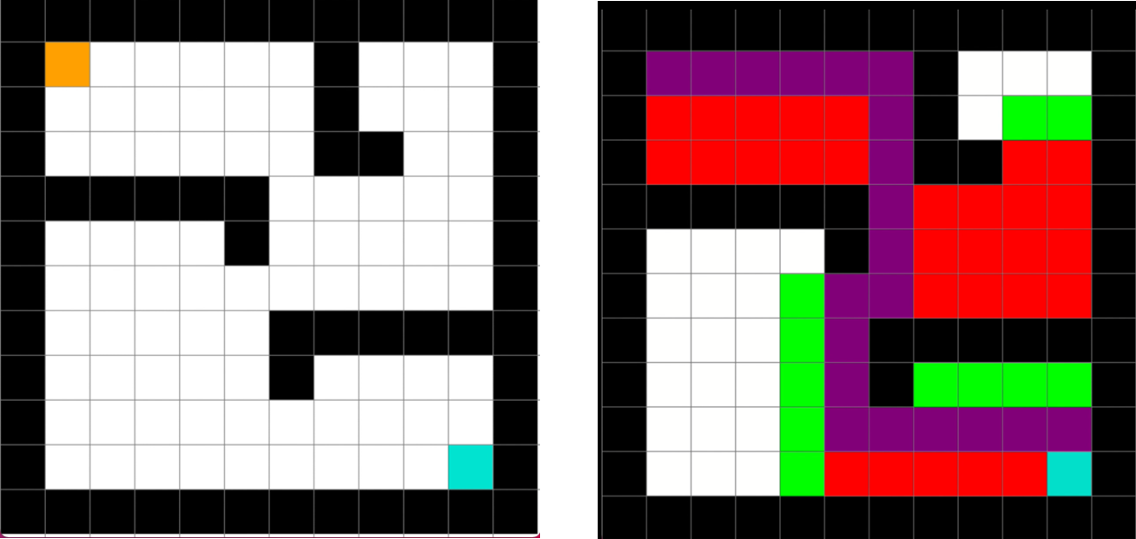
Case Study 2: A Maze with Obstacles

Let’s increase the complexity with a maze that includes internal walls.

• Search Solution: The algorithm, using a heuristic like Manhattan distance, efficiently finds an optimal path from start to finish, navigating around the obstacles. The visualization shows the final path, along with the nodes had to explore to find it.

  

• Reinforcement Learning Solution: The RL agent, using the same sparse reward function as before, learns through trial and error. Initially, its random exploration will cause it to bump into walls repeatedly. Over time, the Q-values for actions leading into walls will remain low (or become negative if a penalty is introduced), while the values for paths leading around the walls towards the goal will increase.

  

The learning curve is similar to the empty grid case, though it may take more episodes to converge due to the increased complexity. The final learned policy provides a comprehensive map for navigating the entire maze from any open square.

The underlying Q-table reflects the structure of the maze. For a state adjacent to a wall, the Q-value for the action that would move into the wall will be extremely low, ensuring the policy guides the agent around it.

State	Up	Right	Down	Left
(1, 2)	0.358	0.397	0.397	0.000
(1, 3)	0.377	0.418	0.418	0.000
…	…	…	…	…
(1, 6)	0.440	0.488	0.000	0.000
…	…	…	…	…
(2, 6)	0.463	0.513	0.000	0.463
…	…	…	…	…

Notice in the table, for state (1, 6), the value for moving ‘Down’ is 0.000. This corresponds to a location in the maze where moving down would hit the horizontal obstacle, correctly identifying it as a poor action. This demonstrates how the Q-function learns the “rules” of the environment implicitly through interaction.

Adversarial Search vs. Reinforcement Learning

We now shift our focus from single-agent navigation problems to two-player, zero-sum games. In this context, the “environment” is no longer static; it includes an opponent whose actions directly counteract our own. This introduces a new layer of complexity and provides another lens through which to compare search-based and learning-based approaches. We will use the game of Tic-Tac-Toe as our primary example.

In an adversarial game, the agent’s goal is to win. The state of the environment is the configuration of the game board. The agent-environment interaction loop remains the same, but the environment’s response to our agent’s action is determined by the opponent’s subsequent move.

Previously, our search algorithms (Minimax, Alpha-Beta Pruning) operated solely on the rules of the game, exploring the game tree to find an optimal move without any external domain knowledge. We could enhance these algorithms with an evaluation function, but that requires hand-crafting domain expertise. Reinforcement Learning offers an alternative: can an agent learn an evaluation function (in the form of Q-values) on its own, simply by playing the game?

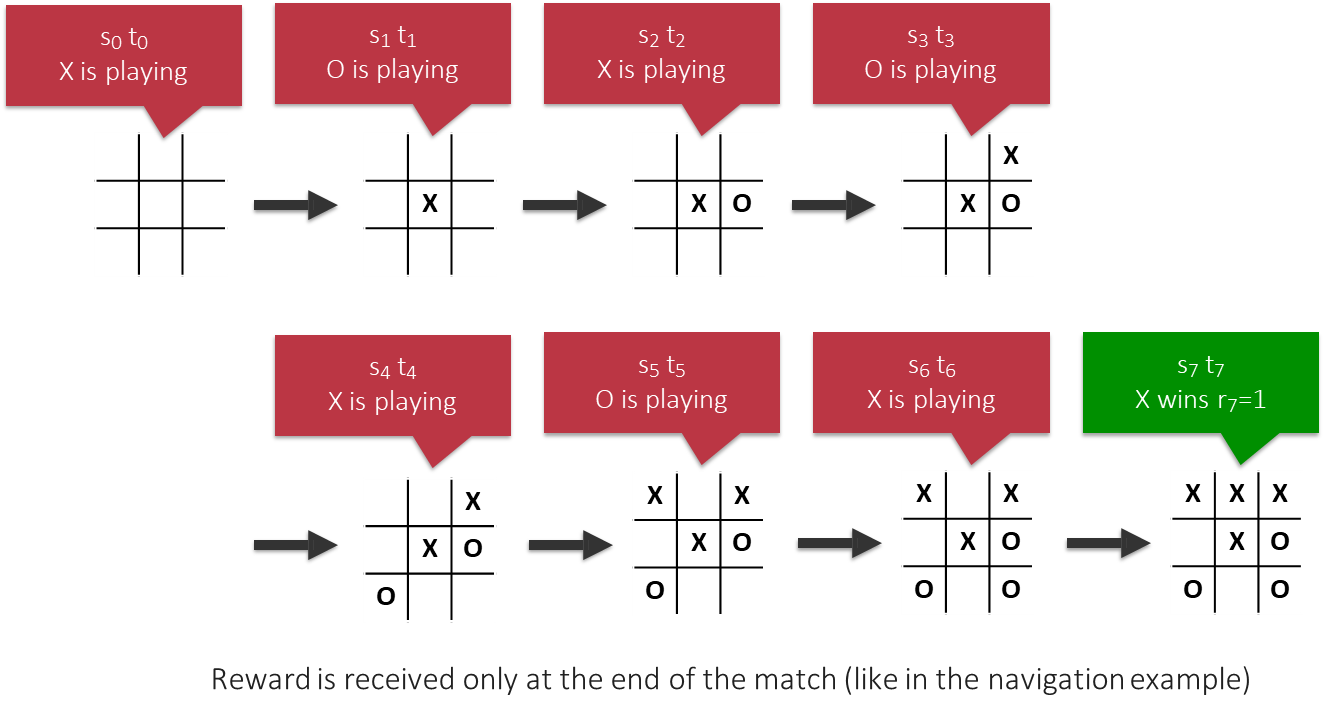
Let’s define the Tic-Tac-Toe problem from a Q-learning perspective. We will train an agent to play as the first player ().

• State (): The current configuration of the 3x3 board.
• Actions (): The set of possible moves, corresponding to the empty squares on the board (up to 9 actions).
• Reward Function: The reward is received only at the end of the game (an episodic task).
  • +1 if the agent wins.
  • -1 if the agent loses.
  • 0 for a draw or any non-terminal move.
• Key Parameters:
  • Learning Rate (): Controls the step size of Q-value updates.
  • Discount Factor (): Determines the importance of future rewards.
  • Initial Q-values (): The value used to initialize the Q-table, often set to 0.

The diagram below illustrates a single episode. The agent () and opponent () take turns, transitioning through states. The reward is only delivered at the final step, , when wins. This delayed reward must be propagated back to all the preceding state-action pairs that contributed to the victory.

A critical challenge in this setup is that the agent’s learning is deeply intertwined with the opponent’s strategy. When our agent is in state () and takes action (), the resulting state () (after the opponent’s move) is not deterministic. It depends entirely on how the opponent plays.

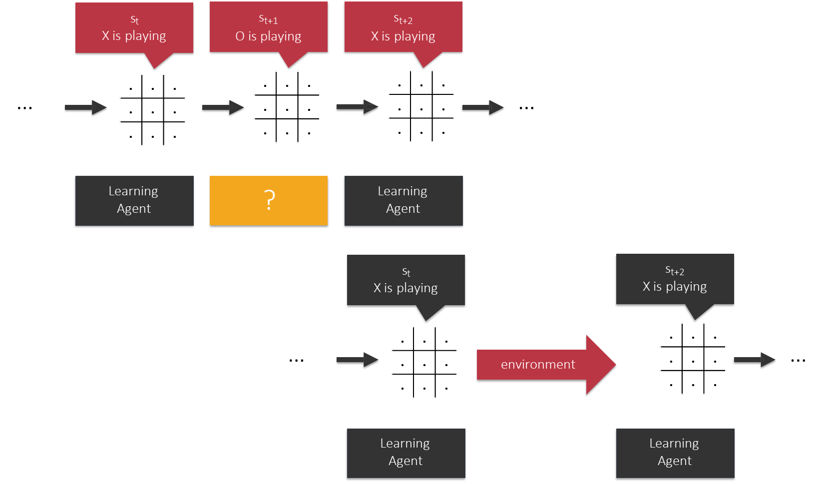
This raises two crucial questions:

1. How do we track performance? We need a consistent metric, like win/loss/draw percentage over a sliding window of games.
2. Who is playing the opponent? The choice of opponent is not just a detail—it is the learning environment. The agent will learn a policy that is optimal against that specific opponent.

Training Scenarios and Experimental Results

The following experiments were conducted by Carsten Friedrich and are available on GitHub. The results show the game outcomes (in percentages) over thousands of training games.

Scenario 1: Opponent is an Optimal Minimax Player

• Description: The Q-learning agent (Player 2) plays against a perfect, deterministic Minimax player (Player 1). The Minimax player will always choose the optimal move.
• Hypothesis: How can an agent learn against a perfect opponent that never makes a mistake? The Minimax player’s moves are deterministic, so from the agent’s perspective, the environment is predictable.
• Results:

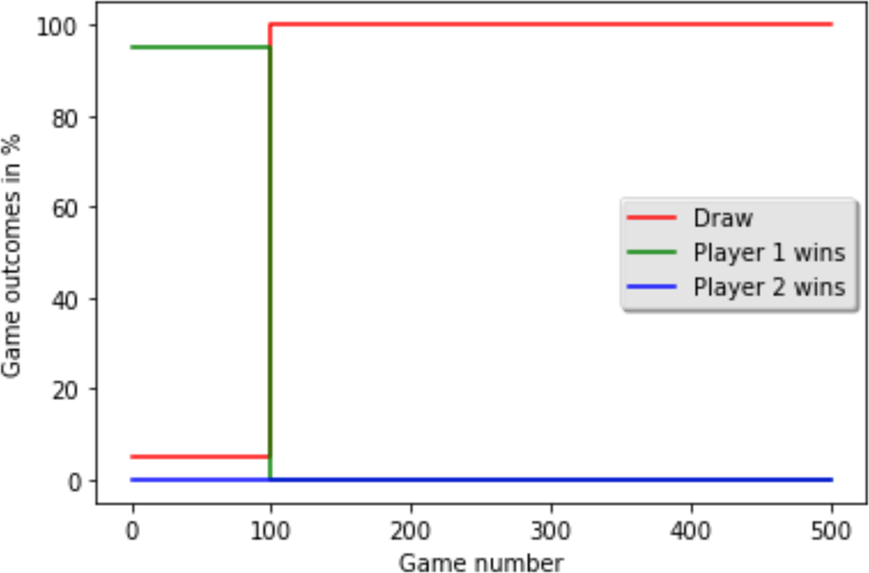
The Q-learning agent fails to learn effectively. After about 100 games, the outcome stabilizes: the Minimax player (Player 1) wins a small percentage of games, and the rest are draws. The Q-learning agent (Player 2) never wins. Because the Minimax opponent is perfect, the learning agent is never “allowed” to win and thus never experiences the +1 reward needed to learn a winning policy. It only learns to not lose (i.e., to force a draw).

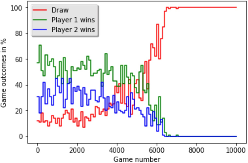
Scenario 2: Opponent is a “Random” Minimax Player

• Description: The opponent still uses the Minimax algorithm to identify all optimal moves. However, if there are multiple moves with the same optimal utility (e.g., several moves that all guarantee a win or a draw), it chooses one of them randomly.
• Hypothesis: This opponent is still optimal but is now stochastic. From the agent’s perspective, taking the same action in the same board state might lead to different next states, depending on the opponent’s random choice. This variability might provide a richer learning signal.
• Results:

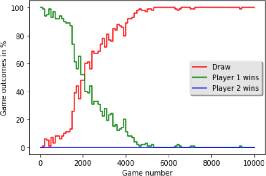
This change has a dramatic effect. The Q-learning agent now learns to play optimally. Initially, the Minimax player (green line) wins most games. However, as the Q-learning agent plays more games, it begins to understand the opponent’s strategy. The number of draws (red line) steadily increases, while the Minimax player’s wins decrease. After about 6,000 games, the Q-learning agent has learned a perfect policy, and every game ends in a draw. The stochasticity provided the necessary exploration for the agent to learn.

Scenario 3: Opponent is another Q-Learning Agent (Self-Play)

• Description: Two Q-learning agents play against each other. Player 1 and Player 2 are both learning from scratch.
• Hypothesis: This is a co-evolutionary process. Initially, both players make random moves, so the game outcomes are erratic. Will they be able to bootstrap their knowledge and converge to optimal play?
• Results:

The learning process is much more volatile. The win percentages for both players fluctuate wildly as they explore the state space and discover new strategies, effectively changing the “environment” for their opponent. For instance, if Player 1 discovers a simple winning trick, its win rate will spike. But then Player 2 will learn to counter that trick, and its own win rate will rise. Eventually, after about 7,000 games, both agents learn the optimal Tic-Tac-Toe strategy, and all games converge to a draw. This “self-play” approach is a powerful concept used in advanced systems like AlphaGo.

Scenario 4: Opponent is a Random Player

• Description: The Q-learning agent plays against an opponent that chooses a valid move completely at random from the available empty squares.
• Hypothesis: This is the weakest possible opponent. It should be easy for the agent to learn to exploit its mistakes.
• Results:

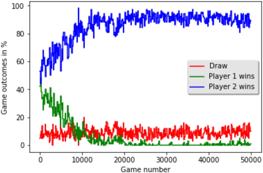
The Q-learning agent (Player 2, blue line) learns very quickly to dominate the random player. Within a few thousand games, its win rate approaches 90-100%. The agent learns an optimal policy against a random player, which in this case is also the globally optimal policy. This demonstrates that RL can learn to exploit a suboptimal opponent’s weaknesses effectively.

Key Takeaways: Minimax vs. Tabular Q-Learning

Feature	Minimax / Alpha-Beta Pruning	Tabular Q-Learning
Feasibility	Feasible for small state spaces. Becomes infeasible even for Connect-4 due to the exponential growth of the game tree.	Feasible for small state spaces where a Q-table can be stored.
Exploration	Explores the entire relevant game tree for each move.	Learns from episodes of play over time.
Optimality	Assumes the opponent plays optimally. It plays optimally from the very first move.	Learns an optimal policy against the specific type of opponent it was trained against. Performance is influenced by the training opponent.
Adaptability	Its value calculation (“at least X”) allows it to exploit a suboptimal opponent’s mistakes.	Needs to be trained, but can learn an optimal strategy against any opponent, even a random one.
Knowledge	Requires only the rules of the game.	Learns a value function (the Q-table) which represents deep, learned knowledge about the game.

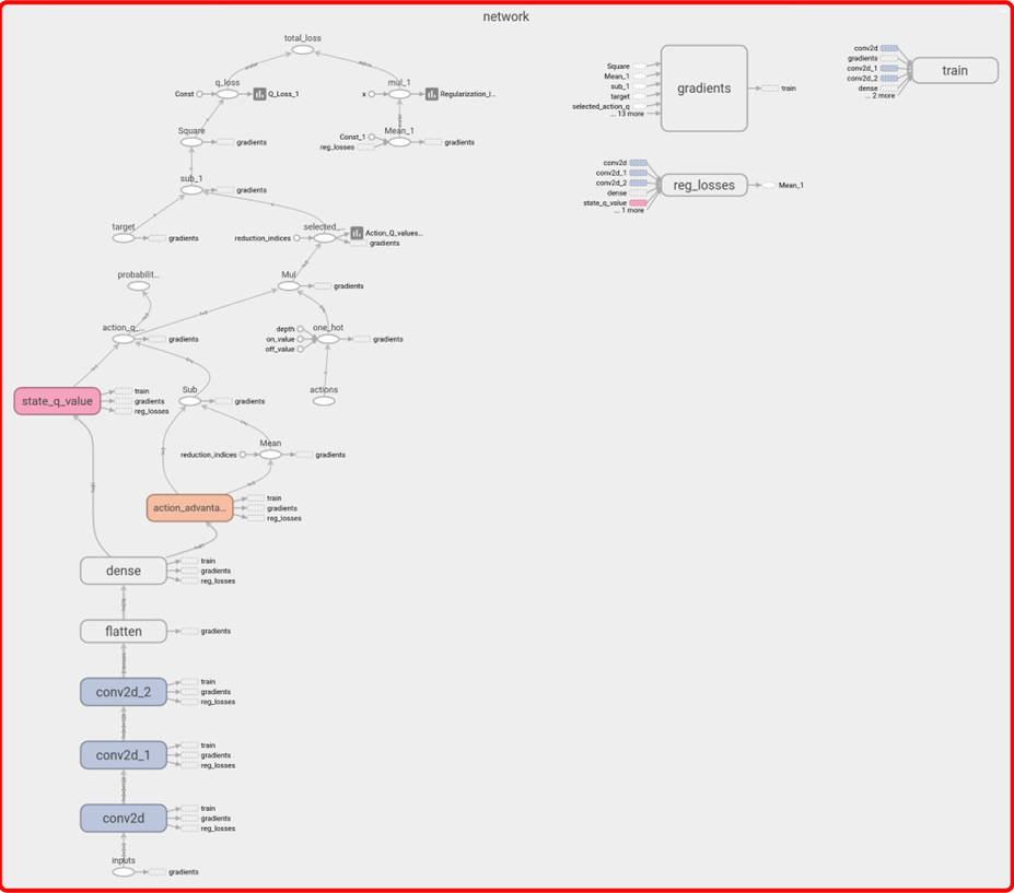
Beyond Tables: Deep Q-Networks (DQN)

As with the navigation problem, the tabular approach for Q-learning is not scalable to games with large state spaces like Chess or Go. The solution is to replace the Q-table with a function approximator, most commonly a Deep Neural Network (DNN). This approach is called a Deep Q-Network (DQN).

• The Q-table is a function mapping (state, action) pairs to Q-values.
• A DNN can be trained to approximate this function. The network takes the game state as input and outputs a Q-value for each possible action.

There is a significant caveat: we are now simultaneously learning the Q-values and learning how to approximate them. This can be unstable, but with modern techniques, it is a highly effective approach.

For a game like Tic-Tac-Toe, a Convolutional Neural Network (CNN) is a natural fit. The input to the network is not just a flat list of squares but a representation that captures the spatial nature of the board. A common technique is to use a multi-channel image-like representation:

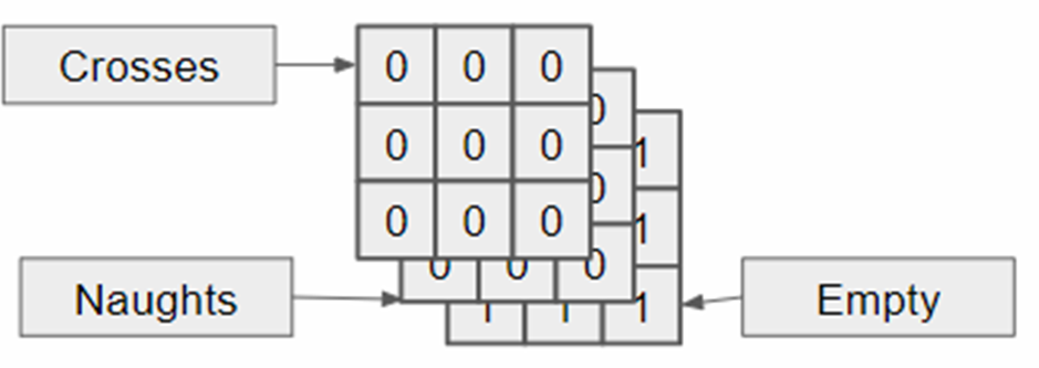
• Channel 1: A grid with 1s where our pieces (Crosses) are, 0s elsewhere.
• Channel 2: A grid with 1s where the opponent’s pieces (Naughts) are, 0s elsewhere.
• Channel 3: A grid with 1s for empty squares, 0s elsewhere (optional, but can be helpful).

This input is then passed through convolutional and dense layers to produce the final Q-values.

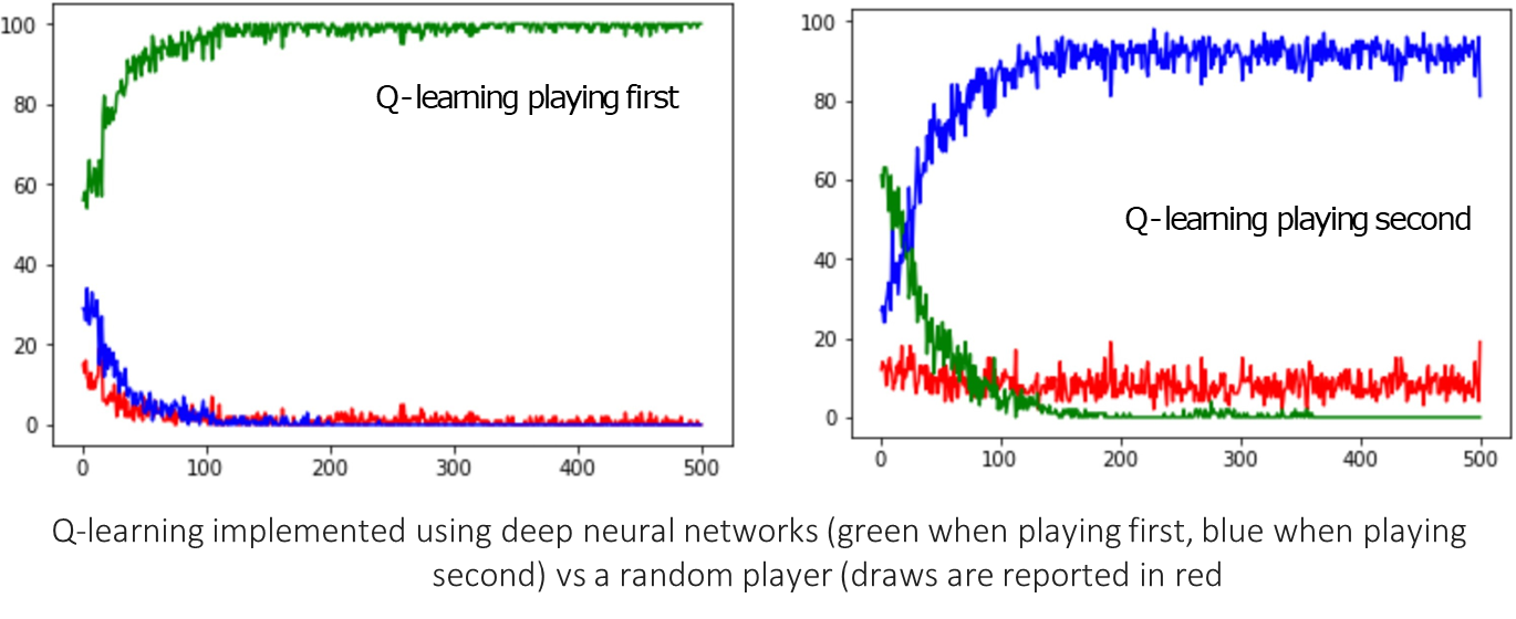
Talking about results, the DQN was trained in two scenarios: against a random player and against a random Minimax player. The performance over thousands of games is shown below.

• DQN vs. Random Player: When playing as either first or second player, the DQN quickly learns to dominate the random player, achieving near 100% win rates. The green line (playing first) and blue line (playing second) show the DQN’s wins, while red shows draws.

  

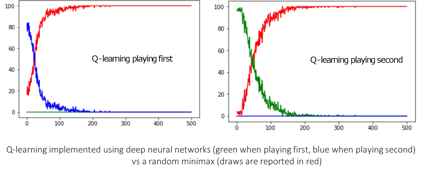
• DQN vs. Random Minimax Player: The DQN also learns to play optimally against the perfect (but stochastic) Minimax opponent. The draws (red line) rise to 100% as the DQN learns it cannot win but can force a draw.

  

These results demonstrate that the principles of Q-learning, combined with the power of deep learning for function approximation, can create highly competent game-playing agents.