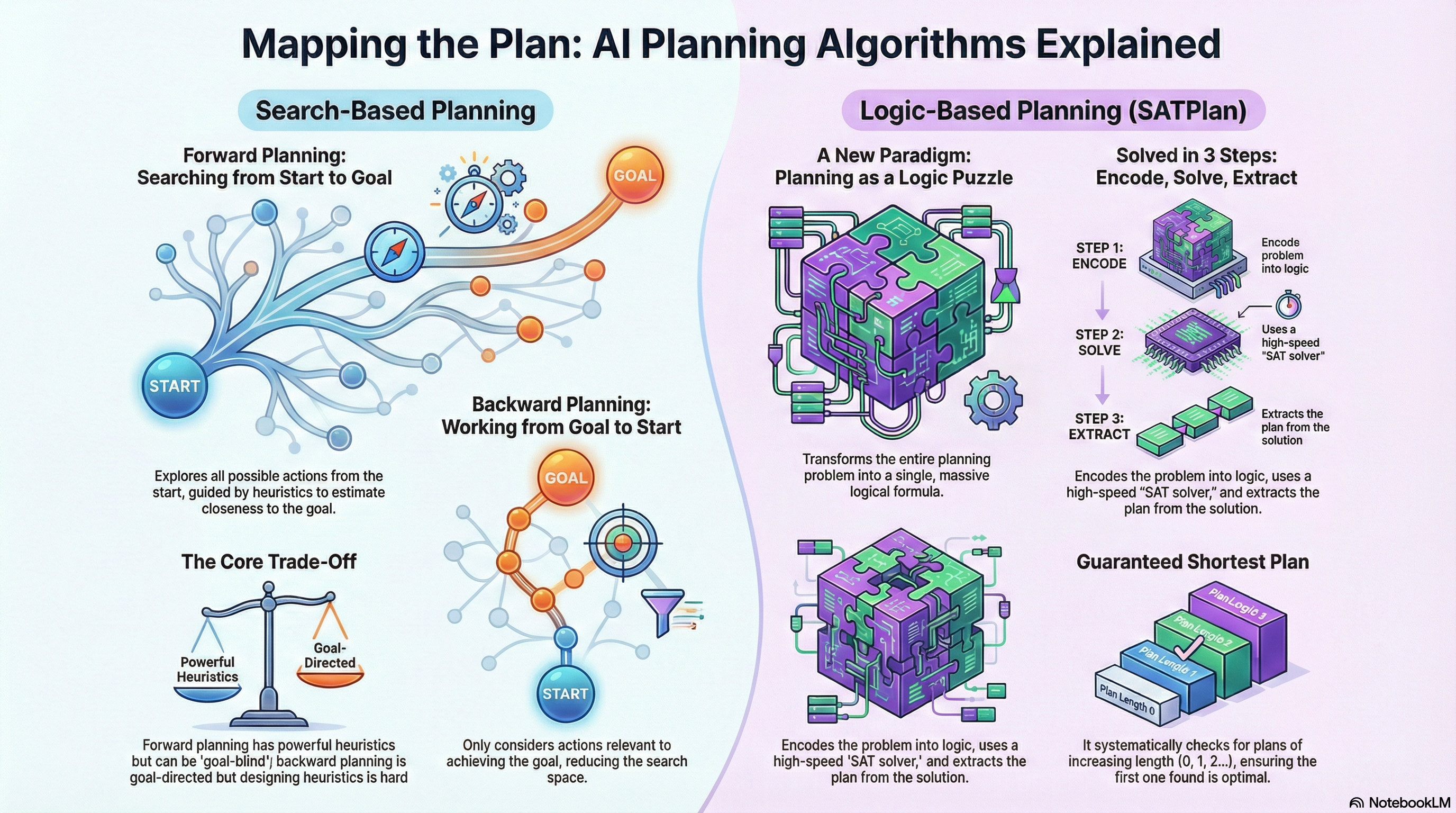
The transition from an abstract search problem to a formal AI planning task requires a precise, structured method for representing the world, the agent’s capabilities, and the desired outcome. This formalization culminates in the definition of a Classical Planning Problem, which is characterized by a deterministic, static, and fully observable environment, utilizing a logical representation for states and effects. This structure is typically captured using formal languages such as STRIPS (Stanford Research Institute Problem Solver) or the contemporary standard, PDDL (Planning Domain Definition Language).
A classical planning problem,
-
The Initial State (
): The World’s Starting Configuration The Initial State is a complete, explicit, and logical description of the world’s configuration at the beginning of the planning process. Within the structured representation context, is defined as a conjunction of ground positive literals—propositions without variables that assert what is true. Critically, the Closed-World Assumption (CWA) is implicitly or explicitly invoked, stipulating that any ground literal not explicitly asserted as true in
is assumed to be false. This simplifies state representation by eliminating the need to enumerate all false facts. -
The Goal Specification (
): The Desired Target State The Goal Specification defines the logical conditions that must be satisfied for the planning problem to be considered solved. The goal is also expressed as a conjunction of literals (which may be positive or negative) that must hold true in the final state. It is important to note that the goal is often a partial description of the world; any state that is reached through a valid plan and satisfies the goal conjunction, , is deemed a valid goal state. -
The Set of Action Schemas (
): The Agent’s Capabilities The set of Action Schemas (or operators) formalizes the agent’s available movements and manipulations within the environment. Each schema is a template defining a class of possible actions, which can be grounded (variables replaced with constants) to form specific, executable actions (e.g., ). This formal definition is typically done using the STRIPS formalism, which consists of three key components for each action schema : - Preconditions (
): A conjunction of literals that must be logically entailed by the current state (i.e., ) for the action to be applicable (executable). - Effects (
): The description of how the world state changes upon execution, divided into: - Add-list (
): A set of positive literals that become true in the successor state . - Delete-list (
): A set of literals that become false in the successor state .
- Add-list (
- Preconditions (
The crucial concept underpinning this formalism is the STRIPS Assumption, which elegantly addresses the computational burden of the frame problem. This assumption states that any fluent not explicitly listed in either the Add-list or the Delete-list of an action remains unchanged by that action. This avoids the necessity of explicitly listing all non-effects (the “frame axioms”) in the action definition.
Given the formal definition
Definition
A solution is formally defined as a finite, ordered sequence of grounded actions
such that, when sequentially applied starting from the initial state , the resultant final state satisfies the goal condition .
The planning problem is thus reduced to a search problem over the vast, implicit space of possible world states reachable through the application of the defined actions.
The central task of any planning algorithm is therefore to effectively and efficiently search this state space—or, alternatively, the space of goals—to discover a valid, and often optimal, sequence of operators. The subsequent exploration of algorithmic strategies, such as forward (state-space) planning (searching from
Plain Planning Algorithms
Following the formal definition of a planning problem, the crucial next phase involves the application of a search algorithm to derive a valid solution plan. The initial, most direct approaches, often termed “plain” or “classical” planning algorithms, are essentially adaptations of traditional state-space search methodologies tailored to the expressive, logical representations inherent in planning domains. These core methods are categorized by their search direction: forward progression from the initial state or backward regression from the goal state.
Comparing Forward and Backward Planning
The two fundamental search methodologies in classical AI planning, Forward (Progression) Planning and Backward (Regression) Planning, present a trade-off between the complexity of the search space and the ease of heuristic design. Modern, efficient planners frequently attempt to synthesize the advantages of both approaches.
Feature Forward (Progression) Planning Backward (Regression) Planning Search Space The complete space of world states. The space of sub-goals (partial world descriptions). Direction Branching Factor High (based on all applicable actions). Lower (based on only goal-relevant actions). Search Guidance Goal-Blind (guided primarily by the heuristic function). Goal-Directed (every step is guaranteed to make progress toward the goal). State/Node Representation Concrete and Complete world state ( ). Abstract and Partial sub-goal specification ( ). Heuristic Design Easier to design strong, admissible heuristics (e.g., ) as they operate on concrete states. Harder to design effective heuristics as they operate on partial, abstract goals. Inconsistency Handling Cannot generate inconsistent nodes (states are complete and consistent). Can generate internally inconsistent sub-goals that may lead to wasted effort if not pruned by external constraints. Backward Planning: Efficiency through Relevance
Backward planning gains a primary efficiency advantage from its inherent goal-directedness. By only considering actions that are relevant—that is, actions whose effects help satisfy some part of the current sub-goal—it often results in a significantly smaller branching factor than forward search. This relevance pruning allows it to quickly focus the search toward the necessary steps. Furthermore, it possesses the capability to prune impossible goals early by failing the consistency check during regression if an action is required to achieve one goal literal but deletes another required goal literal. However, its use of abstract goal representations makes the design of powerful heuristics challenging, and it is vulnerable to exploring long paths resulting from internally inconsistent sub-goals (e.g., requiring the agent to hold two items simultaneously) if such global constraints are not explicitly enforced.
Forward Planning: Robustness through Heuristics
Forward planning’s core strength lies in its concrete state representation, which facilitates the design of powerful and admissible heuristics, such as those derived from the ignore-delete-list relaxation. These strong heuristics, when integrated into an
-like search, can effectively navigate large state spaces. The states are always complete and consistent world configurations, eliminating the concern of exploring internally contradictory nodes. However, its main drawback is the enormous branching factor. Since the search only considers action applicability and not relevance, the planner can be goal-blind, dedicating vast computational resources to exploring actions that are locally valid but entirely irrelevant to achieving the long-term goal.
Forward Planning
Forward planning, or progression planning, represents the most intuitive conceptualization of plan synthesis. The methodology involves searching through the explicit state space, beginning at the defined initial state (
class ForwardPlan(search.Problem):
	"""Forward state-space search"""

	def __init__(self, planning_problem):
		super().__init__(associate('&', planning_problem.initial),
                         associate('&', planning_problem.goals))
		self.planning_problem = planning_problem
		self.expanded_actions = self.planning_problem.expand_actions()

	def actions (self, state):
		return [action
                for action in self.expanded_actions
                if all(pre in conjuncts(state)
                for pre in action.precond)]

	def result(self, state, action) :
		return associate('&', action(conjuncts(state), action.args).clauses)

	def goal_test(self, state):
		return all(goal in conjuncts(state)
				   for goal in self.planning_problem.goals)

	def h(self, state):
		"""
		Computes ignore delete lists heuristic by creating a relaxed version of the original problem
		(we can do that by removing the delete lists from all actions,
		i.e. removing all negative literals from effects)
		that will be easier to solve through GraphPlan and
		where the length of the solution will serve as a good heuristic.
		"""
		relaxed_planning_problem = PlanningProblem(initial=state.state,
                                                   goals=self.goal,
                                                   actions=[action.relaxed() for action in self.planning_problem.actions])
The structured components of the planning problem are directly translated into the elements of a standard search problem
| Search Problem Component | Forward Planning Formalization | Technical Description |
|---|---|---|
| Initial State ( | The initial state | The starting Knowledge Base (conjunction of ground positive literals). |
| Actions ( | The set of all applicable ground actions in state | An action |
| Transition Model ( | The successor state | |
| Goal Test | Check if the current state | The test is successful if all literals specified in the goal |
| Step Cost | A cost function, typically uniform (e.g., 1). | Aims for minimum length plans, favouring breadth-first or A* search strategies over Uniform-Cost Search. |
A critical impediment to the scalability of forward planning is the potential for an enormous branching factor at each state, which stems from the number of applicable ground actions. In domains characterized by a large number of objects and predicates, this set can be prohibitively vast. For instance, in a logistics environment involving
Furthermore, the use of untyped languages (like core PDDL without explicit type hierarchies) can exacerbate this issue by allowing actions to be instantiated with parameters that refer to the same object (e.g.,
Heuristics for Forward Planning
The inherent inefficiency introduced by the high branching factor makes uninformed search strategies largely intractable for real-world planning problems. The key to practical forward planning is the utilization of an informed search algorithm, primarily A*, which requires a domain-specific heuristic function,
The most potent and widely used class of automatically derivable heuristics in planning is based on the concept of solving a relaxed problem. The solution cost of a simplified version of the problem provides a computationally tractable, yet informative, lower bound on the cost of the original problem.
The most effective relaxation is the Ignore-Delete-List Heuristic,
- Actions can only introduce new positive literals (facts).
- Once a fact is asserted as true, it can never be subsequently invalidated or deleted.
- The task is reduced to merely accumulating the necessary set of facts that collectively satisfy the goal
.
The heuristic value
Definition
A heuristic
is considered admissible if it satisfies the condition
for all states
, where is the true minimum cost to reach the goal.
The ignore-delete-list heuristic is provably admissible because:
- Any valid plan
that solves the original problem must necessarily achieve the goal by accumulating all required positive literals. - Because the actions in the relaxed problem have strictly fewer constraints (the non-existence of deletions), the sequence of actions
is also a valid (though possibly suboptimal) solution to the relaxed problem, as the positive literals are still added, and no necessary ones are deleted. - Therefore, the optimal solution length of the relaxed problem,
, cannot exceed the true optimal solution length of the original problem, . Thus, serves as a reliable lower bound on the actual plan cost.
Strengths and Weaknesses of Forward Planning
While being the most straightforward approach, forward planning presents a distinct set of operational trade-offs:
| Category | Strengths | Weaknesses |
|---|---|---|
| Conceptual & Implementation | Intuitive Foundation: Directly maps to established, well-understood search algorithms (e.g., | High Branching Factor: Wastes computational effort exploring a vast number of applicable actions that are ultimately irrelevant to achieving the goal. |
| Performance | High Effectiveness with Heuristics: When coupled with powerful, admissible heuristics (like | Goal “Blindness”: The search direction is determined primarily by action applicability and heuristic estimates, not by explicit relevance to the goal. The planner can easily digress into sequences of applicable, but non-progressive, actions. |
The fundamental limitation of forward planning—its tendency toward goal “blindness” due to the high number of irrelevant applicable actions—is the primary motivation for exploring alternative search methodologies, particularly backward (regression) planning, which is inherently goal-directed.
Backward Planning
In contrast to the state-space exploration of forward planning, backward planning, also known as regression planning, employs a goal-directed search methodology. The core concept involves beginning the search with the ultimate goal specification (
The “state” in this regression search is represented by a set of logical literals (a sub-goal) that must be true at a particular point in time to ensure the final goal is met. The process involves identifying a potential action that could have achieved the current sub-goal and then regressing the sub-goal through that action to determine the necessary predecessor sub-goal. This sequence of regression steps continues until a sub-goal is reached that is already entirely satisfied by the initial state
class BackwardPlan(search.Problem):
	""" Backward relevant-states search """

	def __init__(self, planning_problem):
		super().__init__(associate('&', planning_problem.goals),
                         associate('&', planning_problem.initial))
		self.planning_problem = planning_problem
		self.expanded_actions = self.planning_problem.expand_actions ()

	def actions (self, subgoal):
		"""
		Returns True if the action is relevant to the subgoal, i.e .:
		- the action achieves an element of the effects
		- the action doesn't delete something that needs to be achieved
		- the preconditions are consistent with other subgoals that need to be achieved
		"""

		def negate_clause(clause):
			return Expr(clause.op.replace('Not', ''), *clause.args)
				   if clause.op[:3] == 'Not'
				   else Expr('Not' + clause.op, *clause.args)

			subgoal = conjuncts (subgoal)

			return [action for action in self.expanded_actions
					if (any (prop in action.effect for prop in subgoal) and
						not any(negate_clause(prop) in subgoal
					for prop in action.effect) and
						not any (negate_clause(prop) in subgoal and
						negate_clause(prop) not in action.effect
					for prop in action.precond))]

	def result(self, subgoal, action):
		# g' = (g - effects(a)) + preconds(a)
		return associate('&', set(set(conjuncts(subgoal)).difference(action.effect)).union(action.precond))

	def goal_test(self, subgoal):
		return all(goal in conjuncts(self.goal) for goal in conjuncts(subgoal))

	def h(self, subgoal):
		"""
		Computes ignore delete lists heuristic by creating
		a relaxed version of the original problem
		(we can do that by removing the delete lists from all actions,
		i.e. removing all negative literals from effects) that will be
		easier to solve through GraphPlan and where the length of the
		solution will serve as a good heuristic.
		"""

		relaxed_planning_problem = PlanningProblem(initial=self.goal,
                                                   goals=subgoal.state,
                                                   actions=[action.relaxed() for action in self.planning_problem.actions])
The mapping of the planning problem to a classical search structure in the backward direction is reversed from the forward approach:
| Search Problem Component | Backward Planning Formulation | Technical Description |
|---|---|---|
| Initial State ( | The goal specification | The search starts from the full set of desired final conditions. |
| Actions ( | The set of relevant ground actions that achieve some literal in the current sub-goal | Actions must be chosen based on their ability to make progress towards satisfying |
| Transition Model ( | The new sub-goal | |
| Goal Test | Check if the current sub-goal | The search terminates successfully when the required conditions |
| Step Cost | Typically uniform (e.g., 1). | Aims to find the shortest plan length in terms of actions. |
Relevant Actions and the Regression Operator
The core efficiency gain of backward planning stems from the constrained nature of its action selection: only relevant actions are considered.
Definition
An action
is considered relevant for a current sub-goal if:
- Goal Achievement: At least one literal in
is an element of ‘s Add-list ( ). This ensures the action contributes to satisfying the sub-goal. - Consistency: The action is not inconsistent with
. That is, the action’s Delete-list ( ) does not contain any literal that is also in . If deletes a fact required by the goal, the action is irrelevant, as it moves away from the goal state.
Once a relevant, consistent action
given G and a relevant action A

IF a sub-goal of G is in the delete-list of A THEN RETURN false
G’ ← preconditions of A
FOR EACH sub-goal SG of G DO
	IF SG is not in the add-list of A THEN add SG to G’
RETURN G’
The regression is calculated by the formula:
This formula captures two critical sets of conditions for the predecessor state:
- Action Feasibility: All
must be true to allow the execution of . - Persistent Goals: All literals in
that are not achieved (not in ) must have been true before was executed and must not have been deleted by . The consistency check ensures no required goal literal is in . The resulting set is the new sub-goal to be achieved.
This mechanism immediately prunes paths that involve actions that undo a necessary goal literal, offering a significant advantage over forward search, where such actions may still be applicable.

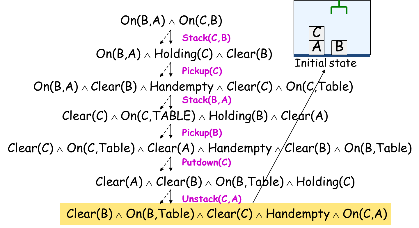
Example 1: Blocks World Regression
The Blocks World scenario demonstrates a successful, multi-step regression to determine the necessary conditions for plan execution.
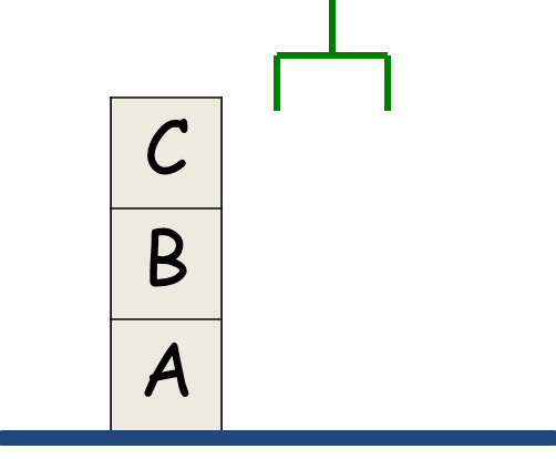
The formal goal
is to have Block B stacked on Block A and Block C stacked on Block B: . The planner selects the action as relevant because its positive effect, , satisfies one of the conjuncts in . The regression
calculates the new sub-goal using the formula:
- Precondition Inclusion: The new sub-goal
must first include the of the action . These are the conditions that must be true in the predecessor state for the action to be legally executed.
- Goal Preservation: The literals in
that are not achieved by the action’s must also be carried over to .
is in the and is thus satisfied by the action. It is discarded. is not in the and is not deleted by the action’s . It must therefore be true in the predecessor state to persist across the action. It is included in . The resulting new sub-goal is
This
is the essential set of conditions that must be met before executing to ensure the ultimate goal is achieved. The search then continues by attempting to find an action that achieves this new sub-goal , effectively moving backward in the plan.
Example 2: Detection of Inconsistent Goals
This example highlights a significant advantage of backward planning: the ability to detect logical impossibilities early through the consistency check inherent in the regression process.
The target goal is
. The planner attempts to use the action to achieve . The inconsistency arises because the action
must not negate any literal required by the goal .
- The goal requires
to be true at the final state. - The
of the action includes . If the action were executed, it would achieve
but simultaneously destroy the required condition . The regression operator fails because the action is inconsistent with the goal. Specifically, the precondition for consistency is . Since , the action cannot be used to achieve . This failure demonstrates that backward search can prune impossible paths before spending excessive computational resources searching for a sequence that would inevitably lead to a contradictory outcome, a form of early dead-end detection.
Challenges and Limitations of Backward Planning
Despite its goal-directed nature and advantage in pruning irrelevant actions, backward planning faces specific challenges related to the abstract nature of its search space:
-
Branching Factor: While often smaller than in forward search, the branching factor can still be substantial. A single literal within a sub-goal can often be achieved by multiple distinct ground actions, leading to a proliferation of successor sub-goals.
-
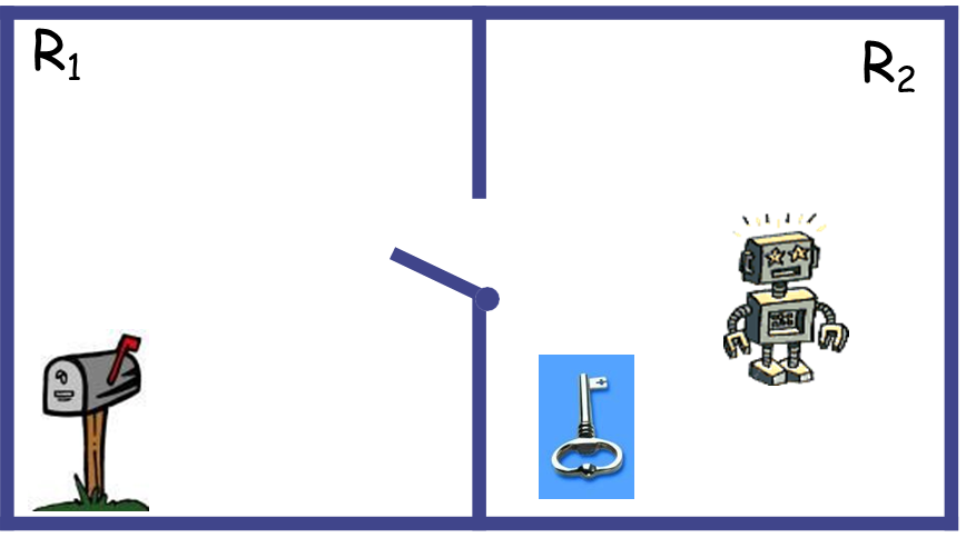
Handling of Internal Inconsistencies (Impossible Sub-goals): A major vulnerability of regression planning is the potential to generate and extensively explore internally inconsistent sub-goals. These are sets of required facts that cannot logically coexist in any single world state (e.g.,
, which violates the constraint that the robot can only hold one item). The regression process itself does not inherently check for the satisfiability of the resulting sub-goal . Without incorporating external state constraints or invariants (axioms defining mutually exclusive conditions, such as ), the planner may waste considerable effort searching along paths derived from an impossible sub-goal. -
Heuristic Difficulty: Developing effective, admissible heuristics
for backward search is typically more complex than for forward search. The “state” is a partial specification (a set of required literals), not a concrete, complete world state. Estimating the minimum number of actions to reach the initial state from a partial goal description is challenging, as the distance is measured to a concrete, fixed set of facts ( ) from a dynamic, underspecified set of constraints.
Backward planning is highly effective due to its relevance pruning, but its susceptibility to generating and failing to detect inconsistent sub-goals, coupled with the difficulty of generating good heuristics, makes it a less common choice in modern optimal planning compared to well-informed forward search.
Efficient Approaches to Planning
While fundamental search paradigms like plain forward and backward planning are essential for conceptual understanding, their efficiency is significantly limited by the combinatorial state explosion inherent in complex domains. To overcome these computational barriers, modern planning research has focused on developing highly efficient paradigms that often re-frame the planning problem into computationally specialized formats for which highly optimized solvers already exist. Key among these efficient approaches are SATPlan, GraphPlan, and Hierarchical Planning.
SATPlan: Planning as Satisfiability
Summary of SATPlan
The SATPlan methodology constitutes a profound paradigm shift in AI planning, moving the problem from the realm of specialized graph search to the robust domain of logical inference and constraint satisfaction.
The core principle is fundamentally a declarative transformation:
Starting from a planning problem formally defined in PDDL, the planner constructs a single, comprehensive knowledge base in Propositional Logic, structured by time-stamped axioms, such that the existence of a satisfying assignment (a model) within this logical representation is computationally equivalent to the existence of a valid plan that solves the initial planning problem.
Key characteristics highlight its effectiveness and theoretical elegance:
Declarative and Formal Representation: The problem dynamics, including action effects and persistence, are fully specified through a finite set of Successor-State Axioms and Precondition Axioms. This provides a transparent, verifiable, and highly formal model of the domain.
Leveraging High-Performance Solvers: By translating the problem into an instance of Boolean Satisfiability (SAT), SATPlan leverages decades of sophisticated research and engineering embodied in modern SAT solvers, which are among the most highly optimized general-purpose constraint solvers available.
Guaranteed Optimality: The employment of an incremental model checking strategy—testing plan length
sequentially—ensures that the first valid plan found is guaranteed to be optimal in the number of steps (the shortest plan). Opportunistic Search Strategy: The underlying search process is highly adaptive and goal-directed, utilizing powerful heuristics like unit propagation to simultaneously propagate constraints forward and backward through time, efficiently converging on a solution or definitively proving non-existence for a given horizon.
These characteristics collectively establish SATPlan and related constraint-based techniques as one of the most powerful and scalable approaches for solving deterministic, classical planning problems, capable of handling complex domains by translating them into a well-understood computational form.
The core innovation of SATPlan is the systematic translation of a classical planning problem into a Boolean Satisfiability (SAT) problem.
Definition
A SAT problem determines whether there exists a truth assignment (a model) for a set of Boolean variables that makes a given propositional logic formula true.
By framing the search for a plan of length
Steps
The process operates via a systematic four-step translation and solving pipeline:
- STRIPS/PDDL to Propositional Logic: The structured domain and problem definition are converted into a vast, single propositional logic formula that simultaneously encodes the initial state, the goal state, and the rules of world change across a fixed number of time steps.
- Conversion to CNF: The propositional formula is transformed into Conjunctive Normal Form (CNF), a conjunction of clauses, where each clause is a disjunction of literals. CNF is the required input format for most high-performance SAT solvers.
- SAT Solver Execution: The CNF formula is submitted to a highly optimized SAT solver (e.g., based on the DPLL algorithm or its modern variants).
- Extraction of the Plan:
- If the solver returns a satisfying assignment (a model), the existence of a valid plan is confirmed. The actual sequence of actions constituting the plan is then read directly from the truth assignments of the action-representing variables in the model.
- If the solver determines the formula is unsatisfiable, it definitively proves that no valid plan of the currently tested length exists.
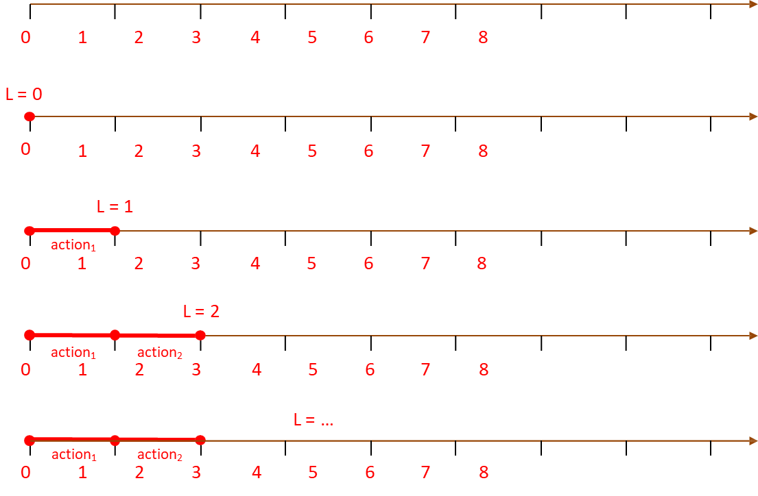
A central challenge for SATPlan is the fixed time horizon required by the propositional encoding. Since the formula must encode the world’s dynamics over a specific number of steps, and the optimal plan length is unknown a priori, SATPlan employs a method analogous to Iterative Deepening Search called Incremental Model Checking.
The strategy systematically searches for the shortest possible plan, guaranteeing optimality in terms of plan length:
-
Set Plan Length
: The process begins with . -
Generate Propositional Formula (
): A formula is constructed, asserting the existence of a valid plan of length
that connects the initial state to the goal . -
Check Satisfiability: A SAT solver checks the formula
. -
Evaluation and Iteration:
- Satisfiable: A solution (model) is found. A shortest plan is extracted from the truth assignments, and the search terminates.
- Unsatisfiable: No plan of length
exists. The length is incremented to , and the process returns to step 2 to build a larger formula .
From PDDL to Propositional Logic
Example
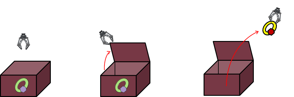
Consider for example the following simple planning problem in which a robot must open a box to retrieve a ring inside it:
- Initial State (
): The box is closed, the ring is inside the box, and the robot’s gripper is free.
- Goal (
): The robot must be holding the ring: . The following actions are available:
- Action 1:
- precondition: box is closed (
); - effect: box is open (
) - Action 2:
- precondition: the ring is in the box and the box is open (
); - effect: the ring is no more in the box and the robot holds the ring (
). The translation process hinges on the introduction of a set of time-stamped propositional symbols to represent fluents and actions at specific points in the planning horizon.
Time-Stamping and Reification
All symbols used in the formula are time-stamped with a superscript
- Fluents: Fluents are state variables (literals whose truth value can change). Each fluent fact
at each time step is represented by a unique propositional variable . For example, is a variable that is true if the box is open at time . asserts that the robot’s gripper is free at time . - Actions (Reification): Actions, which are complex operators in PDDL, are reified (treated as simple propositional variables). An action
at time is represented by a variable . For example, is true if the action is executed between time and .
The Grounding Principle
The complexity of the translation arises from grounding: a propositional variable must be created for every possible ground instance of every predicate and every action schema. If a domain has
Abandonment of the Closed-World Assumption (CWA)
Note
It is crucial to note that the classical propositional logic used in SAT solvers does not adhere to the Closed-World Assumption (CWA) common in PDDL. In propositional logic, a fact is only true or false based on the variable assignment; if a literal is not asserted as true, it is not automatically false. Therefore, the initial state definition must explicitly assert the falsity of all fluents that are false in
. For example, if the box is initially closed, the formula must contain to explicitly constrain the initial state.
This systematic temporal and logical translation allows the entire dynamic planning problem to be encoded as a single, static logical assertion, whose satisfiability search simultaneously solves for the correct action sequence and the resulting state transitions. The next logical step is to explore the axioms that define the constraints and dynamics within this formula.
In our example, what we obtain after grounding and time-stamping is the following translation:
| Original PDDL Element | Propositional Logic Representation | Meaning |
|---|---|---|
| Box | ||
| Box | ||
| Ring | ||
| Robot holds ring | ||
| Robot’s gripper is free (not holds) at time | ||
| Action of opening box | ||
| Action of picking ring |
Constructing the Propositional Formula for SATPlan
The core mechanical brilliance of SATPlan resides in its capacity to translate the complex temporal and causal logic of a planning problem into a massive, static propositional logic formula (a single Knowledge Base,
Formula
The complete formula
for a plan of length is a conjunction of five axiom types:
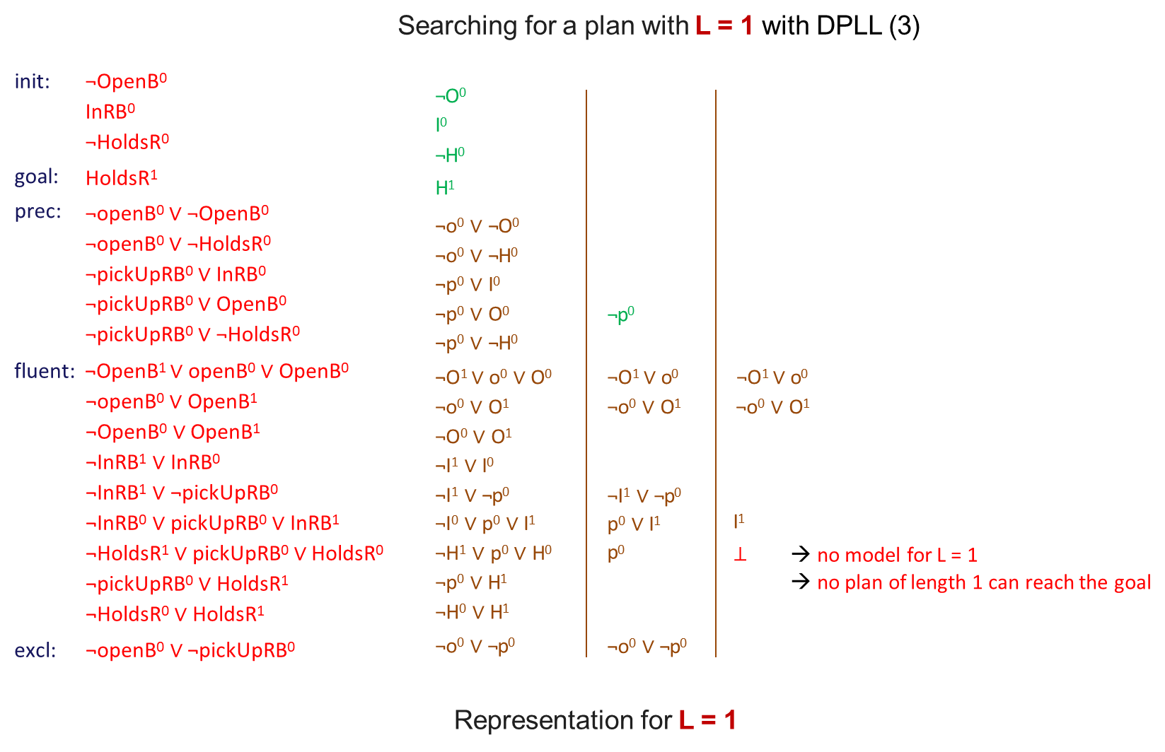
Representation for Plan Length
The base case,
-
Initial State Axioms (
): These explicitly assert the truth values of all fluents at , including negations (due to the lack of the CWA). -
Goal Axioms (
): These assert the goal must be true at .
The complete formula for
Satisfiability Check:
Since the formula explicitly requires both
and to be simultaneously true, the resulting conjunction is an inherent contradiction: . The formula is unsatisfiable, proving that a plan of length zero does not exist, and the SATPlan loop must increment .
Representation for Plan Length
For
Precondition Axioms
Definition
Precondition Axioms specify the necessary conditions for an action to be executed at time
.
These axioms enforce the fundamental rule of action execution: an action can only be executed at time
Example:
- PDDL Preconds:
(which is ) - Axiom:
To obtain the required CNF, the implication
Example
For the
example, this yields three clauses:
Fluent Axioms (Effect and Frame Axioms)
Definition
Fluent Axioms (Effect and Frame Axioms) specify the conditions under which fluents change their truth values from one time step to the next.
These are the most complex and critical axioms, as they define the complete world dynamics, effectively solving the frame problem within the logical formalism. They specify precisely when a fluent
This is the general form of the Successor-State Axiom (SSA). It states that
- an action that adds
was executed at time , or was already true at time and no action that deletes was executed at time .
Example: Fluent
(Ring in Box)
Actions that ADD
: None in this simple model. Actions that DELETE
: .
This yields three CNF clauses:
These SSA clauses must be instantiated for every fluent and for every time step
from to .
Action Exclusion Axioms
Definition
Action Exclusion Axioms specify constraints on the simultaneous execution of actions at the same time step.
These axioms enforce domain-specific constraints on simultaneous action execution. While the SSA and Precondition Axioms already prevent the execution of two actions if they are inconsistent (e.g., if
- Single Action Constraint: To enforce the common classical planning assumption that only one action can be executed at any given time step
. For a set of ground actions, this requires pairwise mutual exclusion clauses of the form: - Mutex Effects: To explicitly forbid two actions whose effects are inherently contradictory (e.g.,
adds and deletes , or adds and adds ), even if their preconditions could be simultaneously met.`
The action exclusion axiom for our example, which prevents simultaneous execution of the two ground actions:
By conjoining the Initial State, Goal, Precondition, Fluent, and Exclusion axioms, SATPlan transforms the search for a plan into a decisive check for the satisfiability of a monumental, yet structured, logical formula.
SATPlan in Action: A Worked Example
Having established the theoretical framework and the requisite axiom categories, we now turn to a concrete application of the SATPlan methodology. We revisit the specific scenario involving a robot, a ring, and a box to demonstrate how the logical machinery processes a planning problem.
The problem is defined by the Initial State at
, where the box is closed, the ring is inside the box, and the robot’s gripper is free
and the Goal State, which requires the robot to hold the ring
The SATPlan algorithm begins its incremental search. As established in the previous section, the attempt for plan length
is immediately deemed unsatisfiable because the initial state does not entail the goal ( ). Consequently, the planner advances to a horizon of . Refutation of Plan Length
For a plan horizon of
, the system constructs a propositional formula attempting to validate the existence of a single action that transitions the world from to . This formula aggregates the initial state axioms at , the goal axiom at , and the full suite of precondition, fluent, and exclusion axioms bridging and . The evaluation of this formula by a SAT solver, typically utilizing the DPLL (Davis-Putnam-Logemann-Loveland) algorithm or a CDCL (Conflict-Driven Clause Learning) variant, proceeds through a sequence of logical deductions. The process initiates with Unit Propagation, where the solver accepts the unit clauses—literals that must be true—as facts. Specifically, the initial state definition fixes
(the box is closed) and the goal definition fixes (the robot must hold the ring at the end). From these fixed points, the solver attempts to construct a valid model through inference. The logical chain proceeds as follows: to satisfy the condition
, the fluent axiom for “holding” is consulted. This axiom dictates that for the robot to hold the ring at when it was not holding it at , the action must have been true. However, the Precondition Axiom for
asserts that this action implies the box was open at ( ). This derivation creates a direct conflict with the initial state axiom . The solver detects this logical contradiction ( ), rendering the entire formula unsatisfiable. This mathematically proves that no single action can solve the problem, prompting the planner to increment the horizon to .
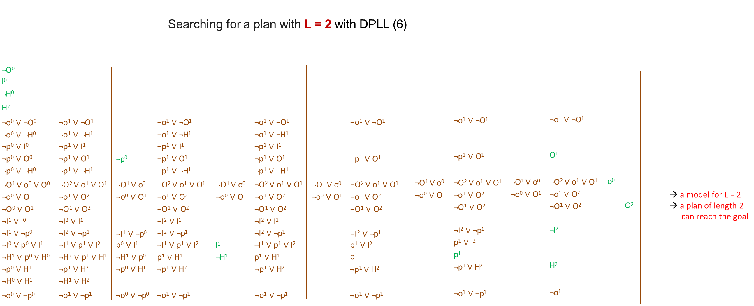
Validating Plan Length
With the horizon extended to
, the propositional formula is expanded significantly. It now encompasses logical constraints for two transition steps:
- from
to , and - from
to . The goal condition is shifted to require satisfaction at
( ), while the intermediate state at is left open to be determined by the solver. The DPLL search initiates again with unit propagation fixing the initial state at
and the goal at . Unlike the previous iteration, the deduction chain does not immediately hit a contradiction. The solver must perform a search by branching on variables—essentially “guessing” a truth value for a variable and propagating the consequences. Suppose the solver branches on the action variable
, assigning it to true. This assignment triggers a cascade of successful implications via the Successor-State Axioms:
- Effect Propagation: Because
is true, the fluent axiom for the box’s status dictates that becomes true (the box is open at ). - Precondition Satisfaction: With
established, the preconditions for the action are now satisfied. - Goal Achievement: The goal
requires a transition from not holding to holding between and . The solver identifies that assigning to satisfies this requirement. - Consistency Check: The solver verifies that no exclusion axioms are violated (e.g., ensuring no other conflicting action is executed at
or ). By finding no contradictions, the solver returns Satisfiable. This indicates that a consistent model—a valid set of truth assignments for all variables across the timeline—has been discovered.
Extraction of the Plan from the Model
The output of the SAT solver is a “model,” which is a raw listing of the boolean value (True/False) for every propositional variable in the formula. This includes every fluent and every action instantiation at every time step. To reconstruct the high-level plan, the algorithm filters this model, specifically isolating the Action Variables that were assigned a value of True.
The interpretation of the model for our scenario yields the following sequence:
- Time Step 0: The variable
is True. This corresponds to the action . - Time Step 1: The variable
is True. This corresponds to the action .
Thus, the extracted solution is the sequence
Analyzing the Search Strategy of SATPlan
Analyzing the search performed by the DPLL-based SAT solver reveals a strategy that transcends the traditional classification of purely forward (progression) or purely backward (regression) search. The search is not governed by the temporal structure of the plan’s timeline, but rather by the logical structure and constraints of the propositional formula itself.
The search strategy employed by the SAT solver is best characterized as opportunistic and constraint-driven. It operates by focusing its deductive efforts wherever the logical constraints are tightest, moving non-monotonically through the time steps
The process begins by immediately establishing constraints at both ends of the timeline due to the Initial State Axioms at
- Forward in Time (Progression): A true action variable
implies a change in state fluents at (via Fluent Axioms). - Backward in Time (Regression): A required state fluent
implies a necessary precondition or a necessary action (also via Fluent Axioms).
The primary engine driving this rapid constraint satisfaction is the Unit Clause Heuristic (or Unit Propagation) within the DPLL algorithm. This heuristic mandates that if any clause in the CNF formula reduces to a single unassigned literal (a unit clause), that literal must be assigned the value that satisfies the clause. This often triggers a powerful cascade of propagation, rapidly constraining the remaining unassigned variables regardless of whether they represent facts near the beginning, middle, or end of the plan. When all unit propagations stall, the solver resorts to the split rule, making an arbitrary choice (a guess or branching point) that restarts the propagation process, thereby exploring the search tree of possible plans.
This opportunistic approach is a critical source of SATPlan’s efficiency. It allows the solver to effectively simultaneously combine the advantages of forward and backward reasoning by focusing on the most informative logical dependencies first. It is a problem-independent heuristic, deriving its power solely from the declarative structure of the constraint network, rather than relying on domain-specific knowledge or goal-distance heuristics.
Planning Graphs and GraphPlan
While SATPlan leverages the raw power of general-purpose logic solvers, an alternative approach involves constructing a specialized data structure that explicitly captures the reachability of states and the necessary sequencing of actions. This structure is known as a Planning Graph, and the algorithm that utilizes it is GraphPlan.
GraphPlan offers a middle ground between the state-space search of forward planning and the logical satisfiability of SATPlan. It works by constructing a directed, layered graph that approximates the planning problem. This graph can be used in two ways: to extract a solution directly (the GraphPlan algorithm) or to derive powerful heuristics for state-space search planners.
Definition
A planning graph is a directed, leveled graph that alternates between State Levels (propositions) and Action Levels.
- Levels: The graph is organized into a sequence of levels
.
- State Level
: Contains nodes representing all literals (positive and negative) that might be true at time . - Action Level
: Contains nodes representing all actions that are applicable given the propositions in . - Edges:
- Precondition Edges: Connect proposition nodes in
to action nodes in . If an action requires a proposition, an edge is drawn. - Effect Edges: Connect action nodes in
to proposition nodes in . Positive effects connect to positive literals, and negative effects to negative literals. - Persistence (No-Op) Actions: To solve the frame problem (representing that things stay the same unless changed), the graph includes specific Persistence Actions (often called No-Ops). For every proposition
in , there is a “No-Op” action in that has precondition and effect in . This explicitly models the choice to do nothing to a variable.
The construction of this graph is polynomial in size relative to the problem definition, making it much smaller than the exponential state space required by standard search. However, the graph is an optimistic approximation: just because a proposition appears in level