The pursuit of building rational agents capable of sophisticated reasoning and autonomous decision-making constitutes a fundamental goal within Artificial Intelligence. A highly influential and powerful framework for achieving this objective is the paradigm of logical agents. This approach centers on representing the agent’s understanding of the world using a formal logical language, which is then actively exploited through defined mechanisms known as inference procedures to derive novel knowledge from existing information.
Definition
A logical agent is fundamentally an intelligent system distinguished by its utilization of a formal logical language to model its internal understanding of the environment, encompassing both static world states and possible actions. This structured, internal model is formalized as a Knowledge Base (KB).
Crucially, the KB is far more than a simple, passive repository of initial facts; it is the dynamic foundation for the agent’s intellectual activities. The agent actively engages with its KB, employing logical reasoning—the application of inference procedures—to deduce information that is not explicitly asserted, thereby expanding its knowledge and ultimately informing its executive function, which dictates the agent’s subsequent course of action in the environment.
The foundational elements that define this logical paradigm is the Logical Sentence (Well-Formed Formula - WFF). This is a statement rigorously expressed within the formal syntax of a particular logical system. For a construct to qualify as a valid logical sentence, it must strictly adhere to the established syntactical rules of the logic, thus classifying it as a well-formed formula (WFF). The expressiveness of the representation hinges on the choice of the logical system.
Propositional Logic (PL):
This is the simplest logic, wherein the fundamental atomic unit is the proposition—a statement that possesses a definite truth value (either true or false). PL primarily focuses on combining these atomic propositions using a set of basic logical connectives such as conjunction ( or AND), disjunction ( or OR), and negation ( or NOT).
First-Order Logic (FOL) / Predicate Logic:
Representing a significant extension of PL, FOL incorporates the notions of variables, objects, predicates and quantifiers. This richer formal structure allows for more complex, expressive, and detailed representations of the world, enabling statements about properties of objects and relations between them.
Modal Logic:
This is a diverse family of logical systems designed to deal with modalities, which are qualifiers that express how a proposition is true. Common modalities include necessity (), possibility (), and epistemic modalities concerning an agent’s belief or knowledge.
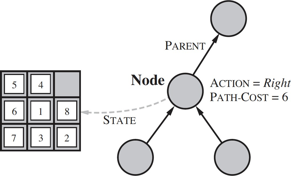
In earlier studies of AI, particularly within the context of search algorithms, the central concept was the state. The standard Node data structure within a search tree traditionally encapsulates an abstract state, along with metadata such as its parent node, the preceding action, and the cumulative cost. The sophistication of state representation can be characterized along an evolutionary continuum, moving from simple, monolithic representations to complex, structured knowledge models.
class Node:
 def init (self, state, parent=None, action=None, path_cost=0):
  """Create a search tree Node, derived from a parent by an action."""
  self.state = state
  self.parent = parent
  self.action = action
  self.path_cost = path_cost
  self.depth = 0

  if parent:
   self.depth = parent.depth + 1
Initially, a system might employ an unstructured state, where the state lacks internal composition and is represented by a single, indivisible descriptor (e.g., the mere name of a city in a simplified route-finding problem). The complexity then increases to a structured state, often seen in Constraint Satisfaction Problems (CSPs), where the state is precisely defined by a collection of distinct variables and their corresponding assigned values. In its most advanced form, integral to the logical agent paradigm, the agent’s complete internal state is its Knowledge Base (KB). This KB is a comprehensive and structured collection of logical sentences that collectively represent all information the agent possesses or holds as a belief about the current and potential states of the world. When the agent’s state is a KB, its dynamic “actions” are transformed from mere physical operations into cognitive functions. These functions include adding new logical sentences to its KB based on sensory perceptions (known as telling the KB) or, critically, performing queries (known as asking the KB) to infer new facts and propositions that were previously implicit, thereby directly guiding its subsequent physical or computational moves.
Inference Procedures
The capacity for inference—the process of determining what new information logically follows from a given body of knowledge—is the essential function of a logical agent.
Definition
An inference procedure is a precisely defined algorithm designed to execute this task.
The fundamental goal of any such procedure is to establish whether a specific query sentence, , is a necessary logical consequence of a premise sentence, , which often represents the agent’s entire Knowledge Base (KB).
This crucial semantic relationship is termed entailment, formally denoted as . This notation signifies that in every conceivable model (or possible world/interpretation) where the premiseholds true, the conclusionmust inherently be true as well. An inference algorithm, , seeks to systematically confirm or deny this entailment relationship, and two distinct methodologies have been developed for this purpose.
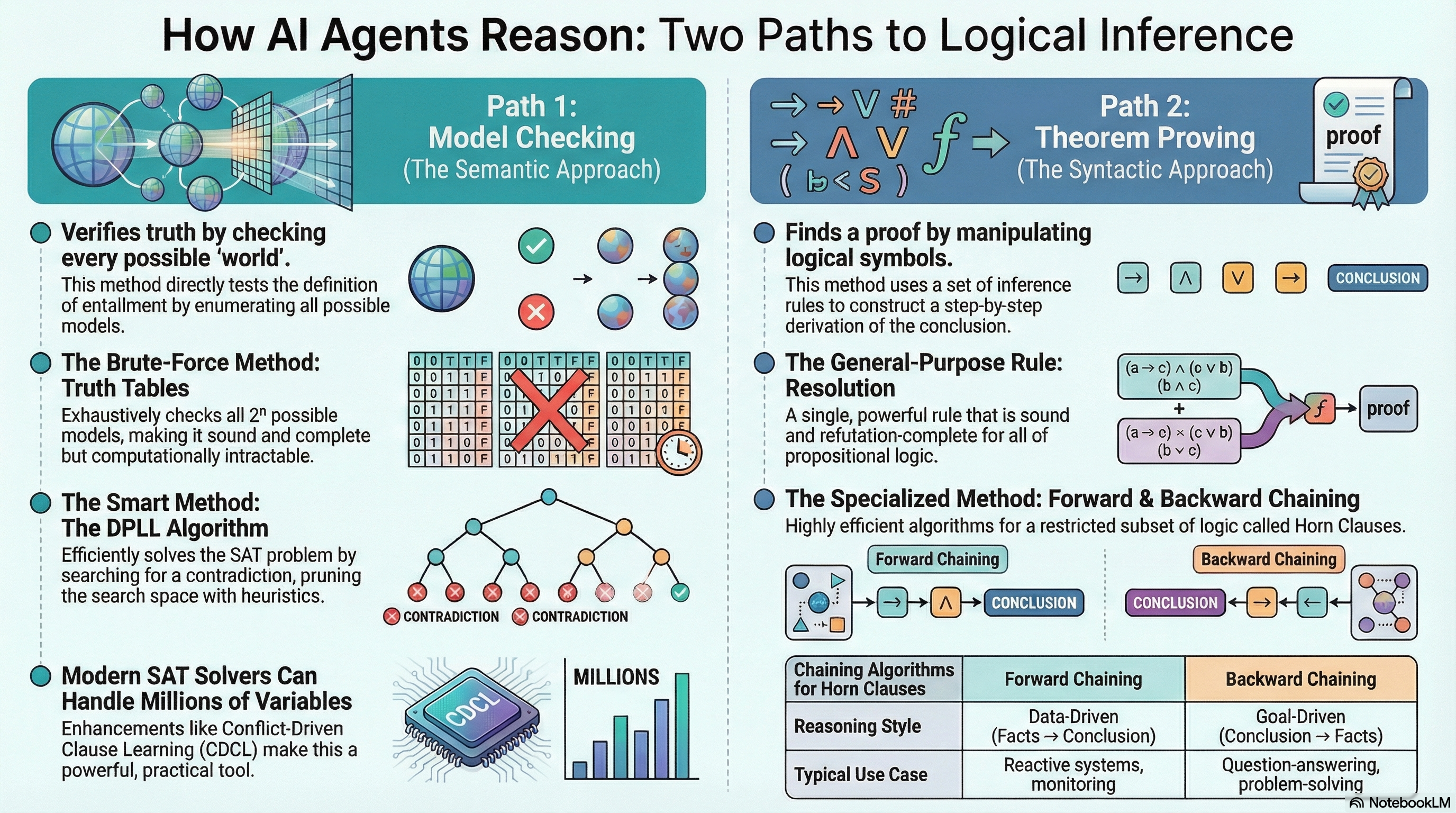
Model Checking
Model checking is an inference technique that rigorously adheres to the semantic definition of entailment. This method directly operates on the semantics—the assigned truth values and meaning—of the logical sentences involved. The process is one of exhaustive verification across the entire space of possible interpretations.
The algorithm’s procedure involves systematically enumerating all possible models relevant to the logical language. A model, in this context, is a complete assignment of truth values to all propositional variables. For each generated model, the algorithm performs two critical checks:
whether the premise evaluates to true, and
if is indeed true, whether the conclusion also holds true within that same interpretation.
The ultimate conclusion of entailment, , is affirmed only if is found to be true in every single model where the knowledge base is true.
Therefore, model checking serves as a systematic, exhaustive search through the space of possible truth assignments, providing a direct, semantic confirmation of the entailment relationship.
Theorem Proving
In contrast to model checking, theorem proving, often referred to as deduction, adopts a purely syntactic methodology. Instead of reasoning about truth values and interpretations (semantics), this approach manipulates the structure and symbols of the logical sentences themselves.
The core of the method is the application of a predefined set of inference rules to construct a formal proof.
Definition
A proof is a finite sequence of logical sentences, where each sentence is either an initial axiom, a sentence from the premise , or a sentence derived from preceding lines in the sequence by the application of one of the established inference rules.
The proof begins with the premise and successfully terminates when the conclusion is derived. If such a construction is successful, we state that is provable or derivable from by the specific algorithm . This syntactic derivation is formally symbolized as .
Soundness and Completeness
The foundational objective in designing robust inference procedures is to ensure a reliable bridge between what is demonstrably provable () and what is genuinely entailed (). The quality of any inference algorithm is rigorously assessed by two key metatheoretical properties: Soundness and Completeness.
Soundness Theorem
An inference algorithm is sound if and only if every sentence it is capable of proving is, in fact, logically entailed by the premise. Stated formally:
Soundness guarantees that the algorithm will never introduce an error; it acts as a reliable filter, ensuring that all conclusions reached through the syntactic process are also semantically true.
Completeness Theorem
An inference algorithm is complete if and only if it is capable of proving every sentence that is logically entailed by the premise. Stated formally:
Completeness ensures the power of the system, guaranteeing that it can theoretically find a proof for any true conclusion.
The ideal standard for a robust inference procedure is to be both sound and complete, which mathematically ensures that the set of sentences that are provable () is perfectly congruent with the set of sentences that are entailed ().
Model Checking Procedures in PL
The task of determining logical consequence, , where a Knowledge Base () entails a sentence , can be resolved using model checking. This is a purely semantic approach that operates by directly implementing the definition of entailment: systematically checking every possible interpretation, or model, of the logical language.
In Propositional Logic (PL), a model is simply a complete and consistent assignment of truth values ( or ) to every propositional symbol present in the and the query .
Reasoning by Truth Tables
The truth table method represents the most direct and conceptually straightforward way to verify entailment. As a form of semantic reasoning, it exhaustively computes the truth value of the and the query under every possible interpretation of the symbols, mirroring the strict definition of entailment.
Algorithm
The process for using truth tables to check is sequential and exhaustive:
Symbol Identification: First, the algorithm identifies the complete set of all distinct propositional symbols (e.g., ) that appear within the ‘s collection of sentences and the query sentence .
Model Enumeration: If unique propositional symbols are identified, the entire space of possible interpretations contains exactly distinct models. These models correspond precisely to the rows of a standard truth table, where each row represents one full truth assignment.
Sentence Evaluation: For every enumerated model (each row of the table), the algorithm calculates the overall truth value of the (which is treated as the conjunction of all its constituent sentences) and the truth value of the query .
Entailment Verification: The final step involves rigorously checking the necessary condition for entailment. The conclusion is that if and only if, in every single model where the evaluates to , the query must also be . Conversely, the existence of even one counterexample model—a row where the is but the query is —is sufficient to definitively prove that the entailment does not hold.
While the truth table method is inherently sound and complete for Propositional Logic, its practical application is severely limited by its computational complexity. The algorithm requires checking rows, where is the number of symbols. Since the satisfiability problem (and thus entailment checking) is co-NP-complete, this exponential complexity makes the brute-force truth table method completely intractable for knowledge bases involving more than a few dozen propositional variables.
Example: The Raincoat Problem
To solidify the understanding of Model Checking via the truth table method, we apply the procedure to the Raincoat Problem. The objective is to semantically prove the entailment: , based on the following premises:
Where the propositional symbols are (), (), and (). With symbols, there are distinct possible models, which are systematically enumerated in the verification table.
The following table evaluates the truth of the two sentences ( and ) and the query () across all eight models:
“When it rains and it is windy, Alice wears a raincoat”:
“It rains, but Alice does not wear a raincoat”:
“Therefore, it is not windy”:
0
0
0
0
1
1
0
0
1
0
0
1
0
1
0
0
0
1
0
1
0
0
1
1
0
0
0
0
1
1
0
1
0
0
0
0
1
0
0
0
1
1
1
1
1
1
0
1
0
1
0
0
0
1
1
1
0
1
0
1
1
0
0
1
1
1
1
1
0
0
0
0
To confirm , one must isolate all KB-models—that is, the rows where the overall conjunction evaluates to True. In this exhaustive enumeration, only the fifth row satisfies this condition: the model where , , and .
In this unique -model, the truth value of the query is also observed to be True. Since the query sentence is in all models (in this case, only one) that make the true, the definition of entailment is satisfied, and we definitively conclude that the entailment holds; thus, it is logically necessary that it is not windy ().
The truth table method, while foundational for understanding entailment, possesses a well-defined set of metatheoretical properties that simultaneously define its power and its limitation:
Property: Soundness and Completeness
This procedure perfectly operationalizes the semantic definition of logical entailment.
It is sound because it guarantees that every conclusion found () is indeed logically entailed ().
It is also complete because it systematically finds every true entailment, ensuring the algorithm does not miss any valid conclusion.
Property: Decidability
In Propositional Logic, the truth table method is decidable. Given a finite number of propositional symbols, the number of models is finite and fixed (). Therefore, the algorithm is guaranteed to terminate after a finite, predictable number of steps, always returning a conclusive or answer regarding the entailment.
Property: Computational Intractability
The primary, crippling drawback is the exponential time complexity of , where is the number of propositional symbols and is the number of sub-sentences in the . This exponential growth rate means the method becomes computationally intractable for knowledge bases exceeding a small number of variables (typically around 20-30), rendering it impractical for real-world AI systems.
Property: Lack of Transparency
The reasoning process is fundamentally brute-force and non-human-like. It provides no intuitive or causal explanation for why the conclusion follows, as a human would using sequential logical steps (e.g., Modus Ponens). This limits its utility in applications requiring a transparent or explainable AI component.
The DPLL Algorithm
The exponential complexity of the exhaustive truth table method, , renders it computationally intractable for knowledge bases of realistic size. Consequently, sophisticated techniques are required, with the most influential being the DPLL (Davis-Putnam-Logemann-Loveland) algorithm.
Idea
DPLL does not check entailment directly; rather, it is an optimized, systematic procedure designed to solve the Propositional Satisfiability (SAT) problem. This problem asks whether there exists at least one complete model (a consistent truth assignment) that makes a given propositional logic sentencetrue. If such a model is found, is satisfiable; otherwise, it is unsatisfiable.
The practical connection between the SAT problem and the core task of entailment checking () is established through the principle of proof by contradiction, also known as refutation.
A fundamental equivalence in logical reasoning states that holds true if and only if the compound sentence is unsatisfiable.
This allows a logical agent to leverage efficient SAT-solvers, like DPLL, to prove entailment. The agent constructs the negation of the query sentence () and conjoins it with its Knowledge Base. If the DPLL solver determines that this combined sentence, , permits no possible model that makes it true—i.e., it is unsatisfiable—then the original entailment is proven.
Although the SAT problem is classified as NP-complete, implying that no polynomial-time worst-case algorithm is known, highly optimized DPLL implementations exhibit remarkable performance on a wide range of practical, non-worst-case instances.
Conjunctive Normal Form (CNF)
A crucial prerequisite for the DPLL algorithm is that the input sentence must be normalized into Conjunctive Normal Form (CNF). This standardized structure simplifies the search space and facilitates the application of powerful pruning heuristics.
Definition
A CNF sentence is defined as a conjunction (, ) of one or more clauses, where each clause is, in turn, a disjunction (, ) of one or more literals. A literal is an atomic propositional symbol (e.g., ) or its negation (e.g., ).
Consequently, a CNF sentence is true if and only if every single clause within it is true, and a clause is true if at least one of its literals is true.
Any propositional sentence can be converted into a logically equivalent CNF sentence via a systematic process involving four primary steps:
Steps
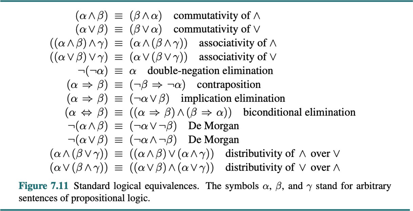
Elimination of Biconditionals and Implications: Logical connectives like (biconditional) and (implication) are eliminated by replacing them with their equivalent conjunctions and disjunctions. For instance, is replaced by , while is replaced with
Internalizing Negations: De Morgan’s laws and the principle of double-negation elimination are applied recursively to move negation symbols () inwards until they only precede atomic propositional symbols.
Distribution: The final step applies the distributivity law (specifically, distributing over ) to transform the sentence into the final CNF format, which is a top-level of terms.
Example
For example consider the following sentence:
The DPLL Search Algorithm and Pruning Heuristics
The DPLL algorithm operates as an intelligent backtracking, depth-first search across the space of possible partial truth assignments. Its goal is to find a set of assignments that satisfies all clauses.
The efficiency of DPLL, and its ability to drastically outperform the brute-force check, stems from its intelligent pruning of the search tree using look-ahead heuristics that deduce logical consequences before resorting to arbitrary branching:
Early Termination: This critical step allows the search to stop immediately along any path if a definitive conclusion is reached:
Success: If the current partial assignment satisfies all clauses, a satisfying model has been found. The algorithm terminates successfully, and the formula is satisfiable.
Failure: If the current partial assignment causes even a single clause to be falsified (meaning all literals in that clause are ), that entire branch of the search space is immediately invalid. The algorithm backtracks to the last decision point, pruning a potentially vast sub-tree.
Pure Literal Heuristic: A pure literal is one whose symbol consistently appears with the same sign (either always positive or always negative) across all remaining unsatisfied clauses.
Action: The algorithm safely assigns the truth value to the pure literal that makes it True. For example, if only appears as (and never ), assigning will satisfy every clause containing it.
Rationale: Since the pure literal cannot contradict any other literal in any remaining clause, this assignment is guaranteed not to close off a solution, serving as a safe simplification that removes satisfied clauses and reduces the search space.
Unit Clause Heuristic (Unit Propagation): A unit clause is a clause containing only one unassigned literal.
Action: This literal constitutes a forced deduction; it must be assigned the truth value that makes it to avoid immediate falsification of the entire clause. For a clause , if is the only unassigned literal, must be assigned .
Rationale: The critical result of this forced assignment is unit propagation, a cascade effect where the new assignment satisfies the unit clause and may subsequently simplify other clauses into new unit clauses, enabling a rapid, deterministic expansion of the partial assignment and significantly reducing the depth of the search required.
If none of these powerful heuristics can be applied, DPLL then resorts to branching, selecting an unassigned variable (often using an auxiliary heuristic) and recursively trying both assignments ( and ) until a solution is found or the search space is exhausted.
function DPLL-SATISFIABLE?(s) returns true or false
	inputs: s, a sentence in propositional logic

	clauses ← the set of clauses in the CNF representation of s
	symbols ← a list of the proposition symbols in s

	return DPLL(clauses, symbols, {})

function DPLL(clauses, symbols, model) returns true or false
	if every clause in clauses is true in model then
		return true

	if some clause in clauses is false in model then
		return false

	P, value ← FIND-PURE-SYMBOL(symbols, clauses, model)

	if P is non-null then
		return DPLL(clauses, symbols - P, model ∪ {P=value})

	P, value ← FIND-UNIT-CLAUSE(clauses, model)

	if P is non-null then
		return DPLL(clauses, symbols - P, model ∪ {P=value})

	P ← FIRST(symbols);
	rest ← REST(symbols)

	return DPLL(clauses, rest, model ∪ {P=true}) or
		   DPLL(clauses, rest, model ∪ {P=false})
DPLL Walkthrough 1: A Satisfiable Case
This walkthrough demonstrates the execution of the DPLL algorithm to determine the satisfiability of the propositional logic sentence set . The initial set is
Step 1: Conversion to Conjunctive Normal Form (CNF)
The initial sentences must first be converted into an equivalent set of clauses in CNF:
Implication Elimination: The conditional sentences are transformed using the equivalence .
(using De Morgan’s Law )
Literal Preservation: The literal is already a unit clause in CNF.
The complete Knowledge Base (KB) in CNF is the set of clauses:
The set of propositional symbols is .
Step 2: Running the DPLL Algorithm
The DPLL algorithm performs a depth-first search, applying unit propagation and pure literal elimination to prune the search space.
1. Unit Propagation
The algorithm first identifies and enforces Unit Clauses, which are mandatory assignments.
Identification: Clause is a unit clause. The literal must be to satisfy the clause.
Assignment: The truth assignment (or ) is mandated.
Model Update:.
Simplification (Unit Propagation):
since (False), the clause simplifies to .
is and satisfied.
is unchanged.
is satisfied because is .
Remaining Clauses:.
2. Pure Literal Elimination
The algorithm next identifies literals that appear with only one polarity in the remaining unsatisfied clauses.
Pure Literal Check in :
appears in and (only negatively). Pure.
appears in (positively) and appears in (negatively). Not Pure.
appears in (only positively). Pure.
Assignment Selection: Let’s select the pure literal . To make True, we must assign (or ).
Model Update:.
Simplification (Pure Literal Elimination):
is satisfied because is .
is satisfied because is .
Remaining Clauses:.
3. Early Termination (Success)
Conclusion: The set of remaining clauses is empty ().
Result: All original clauses have been satisfied by the partial assignment. The algorithm terminates and returns SATISFIABLE.
A minimal satisfying partial model is . Since the algorithm successfully found a model, the original set of sentences is indeed satisfiable. Note that the unassigned variables, and , can be assigned arbitrarily (e.g., ) to form a complete model, .
DPLL Walkthrough 2: Handling a Splitting Case
This walkthrough illustrates the DPLL algorithm’s approach to situations that require branching (splitting) when the deterministic heuristics—Unit Propagation and Pure Literal Elimination—cannot be applied immediately. The goal is to determine the satisfiability of the sentence , which is already provided in Conjunctive Normal Form (CNF):
The set of clauses is , with symbols .
1. Initial State Analysis (No Deterministic Heuristics)
The algorithm first checks for immediate deductions:
Unit Clauses: There are no clauses containing only one literal, so no unit propagation is possible.
Pure Literals:
appears in and (positive) and appears in (negative). Not Pure.
appears in and (positive) and appears in (negative). Not Pure.
Since neither heuristic can simplify the problem, the algorithm must split—a deterministic choice of a variable followed by a recursive search for each of its two possible truth values. We select the variable as the branching variable.
2. Branch 1: The Assumption
The algorithm makes the non-deterministic assumption (or ) and updates the partial model: .
Clause Simplification: Any clause containing is immediately satisfied (True) and can be pruned:
is satisfied (pruned).
is satisfied (pruned).
Clause Reduction: Any clause containing must have eliminated, since is and cannot satisfy the clause:
is reduced to the single literal clause .
Remaining Clauses:.
3. Application of New Heuristics (Unit Propagation)
After the split, the problem is simplified, enabling the application of heuristics:
Unit Clause: The remaining clause is a unit clause.
Assignment: The literal must be to satisfy the clause. We enforce the assignment (or ).
Model Update:.
Remaining Clauses:.
4. Early Termination (Success)
Since the set of remaining unsatisfied clauses is now empty, all original clauses are satisfied by the current truth assignment. The algorithm terminates successfully and reports SATISFIABLE.
A satisfying model has been found: . Crucially, because the goal of the SAT problem is merely to find one such model, the algorithm is not required to explore the second branch (the assumption ). The entire sub-tree corresponding to is implicitly pruned, showcasing the DPLL’s effectiveness in avoiding unnecessary search space traversal.
Advanced Applications of DPLL and Modern SAT Solving
The DPLL algorithm’s capability to determine the Propositional Satisfiability (SAT) status of a formula extends far beyond merely finding a single model. Its true significance in artificial intelligence and formal reasoning lies in its capacity to prove unsatisfiability, which is the computational basis for establishing logical entailment through the method of refutation. Furthermore, modern enhancements have transformed DPLL into the core engine of highly powerful SAT solvers used for complex real-world problems.
The demonstration of unsatisfiability is the cornerstone of proving that a Knowledge Base logically necessitates a conclusion (). As established by the Deduction Theorem (in its refutation form),
is confirmed if and only if the conjoined sentence is unsatisfiable.
The DPLL algorithm proves unsatisfiability by systematically performing a complete, exhaustive search of the solution space and demonstrating that every possible truth assignment leads to a logical contradiction, or the falsification of at least one clause.
Example: Proving Unsatisfiability via Exhaustive Search
Let’s examine the set of sentences .
This set is intentionally constructed to be contradictory. Since the clauses are already in CNF, we proceed directly to the DPLL search with the clause set
on symbols .
Initial Split: As no heuristics apply, the algorithm must split on a variable, say .
Branch 1: Assume ()
Simplification: Clauses and are satisfied. Clauses and are reduced by eliminating (since is ).
Remaining Clauses:.
Conflict: The remaining set immediately contains two unit clauses, and , which demand contradictory assignments: must be to satisfy the first, and must be to satisfy the second. This internal contradiction—a clash between required assignments—falsifies the entire clause set under this branch. The search backtracks.
Branch 2: Backtrack and Assume ()
Simplification: Clauses and are satisfied. Clauses and are reduced by eliminating (since is ).
Remaining Clauses:.
Conflict: Similar to the first branch, the reduced clause set again contains the conflicting unit clauses and . This leads to an immediate contradiction and subsequent backtracking.
Since the DPLL algorithm has definitively explored all possible branches of the truth assignment space ( and ) and found that every path leads to the falsification of a clause (a logical contradiction), the algorithm concludes that the formula is UNSATISFIABLE.
This proof of unsatisfiability, achieved by exhausting the search space without finding a model, provides the computational engine for deductive inference in a logical agent.
Enhancements for Modern SAT Solving (CDCL)
While the original DPLL algorithm is sound and complete, it is the basis for much more powerful modern SAT solvers, which are typically based on the Conflict-Driven Clause Learning (CDCL) paradigm. CDCL builds upon DPLL’s foundation (Unit Propagation and Splitting) by introducing sophisticated techniques that drastically improve performance on hard instances:
Learning:
Upon detecting a conflict (clause falsification), the solver analyzes the chain of decisions and propagations that led to the failure. It then generates a new, non-redundant clause, called a conflict clause, which is logically entailed by the but explicitly prohibits the contradictory assignment that caused the failure. This conflict clause is permanently added to the .
Non-Chronological Backtracking (Jump Backtracking):
Instead of simply backtracking to the most recent decision point (chronological backtracking), CDCL uses the information in the conflict clause to identify the earliest decision point that is responsible for the contradiction. The solver can then jump back to that point, often skipping many intervening layers in the search tree and pruning large, irrelevant sections of the search space.
Variable/Value Ordering Heuristics:
Modern solvers use highly dynamic, sophisticated heuristics to choose the next variable to split on, often prioritizing variables that have recently been involved in conflicts or those that appear frequently in small, critical clauses.
Entailment via SAT
The most efficient and widely used method for a logical agent to prove logical entailment () in Propositional Logic is through proof by refutation using a SAT solver, such as the DPLL algorithm. This technique relies on the fundamental relationship between entailment and unsatisfiability, replacing the exponential semantic search of truth tables with a focused, conflict-driven syntactic search.
The core principle is to construct a test sentence () that represents the negation of the desired entailment and then prove that is logically impossible (i.e., unsatisfiable). The procedure is structured as follows:
Steps
Formulate the Test Sentence ():
The agent constructs the combined sentence . This sentence formalizes the hypothesis that the Knowledge Base is true ( is satisfiable) and the query is false ( is satisfiable).
Conversion to CNF:
The test sentence is converted into an equivalent set of clauses in Conjunctive Normal Form (CNF), a necessary input format for DPLL.
SAT Solver Execution (DPLL):
The resulting CNF clause set is input to the DPLL algorithm. The solver performs a systematic, backtracking search, driven by unit propagation and other heuristics, to find a model that satisfies all clauses.
Interpretation and Conclusion:
If the DPLL solver returns UNSATISFIABLE (), it means the attempt to find a world where is true and is false failed. This contradiction confirms that the original entailment must hold: .
If the solver returns SATISFIABLE (), it has successfully identified a specific counterexample model—a truth assignment where holds but fails. This model proves that the original entailment does not hold ().
We can now use this refutation procedure to formally and efficiently prove the conclusion of the Raincoat Problem: that .
KB Sentences
Query
Goal
Prove
The test sentence is , which simplifies to
The equivalent set of CNF clauses is:
The search begins with the highly constrained environment imposed by the initial unit clauses, , , and .
Forced Assignment (Unit Clause ): forces the assignment .
Propagation: is simplified by eliminating (since is ), resulting in the new clause .
Remaining Clauses:.
Forced Assignment (Unit Clause ): forces the assignment .
Propagation: is simplified by eliminating (since is ), resulting in the new unit clause .
Remaining Clauses:.
Conflict Detection:
The remaining clauses are the two unit clauses, and .
forces the assignment .
This assignment falsifies the clause , as evaluates to .
The DPLL algorithm arrived at a direct logical contradiction (a conflict) entirely through a sequence of forced deductions (unit propagation) without needing to perform any arbitrary splits.
unit clause
✓
unit clause
✓
✓
unit clause
✓
✓
✓
✕
conflict
Since the assignments , , and the resulting conflict were logically necessary to satisfy the starting set of clauses, the contradiction proves that no assignment of truth values can possibly satisfy . Therefore, the test sentence is UNSATISFIABLE, which, by refutation, confirms the logical entailment: .
Efficiency and Practical Applications of Modern SAT Solvers
The transition from the theoretical DPLL algorithm to state-of-the-art SAT solvers represents a profound leap in computational capability. While a basic DPLL implementation might be limited to problems with approximately 100 variables, modern, highly-optimized solvers can routinely handle massive instances involving over 10 million variables. This dramatic increase in efficiency stems from incorporating a collection of sophisticated enhancements that allow solvers to navigate the NP-complete search space far more intelligently than the basic backtracking method.
Modern SAT solvers are fundamentally built upon the DPLL search backbone but augment it with complex, domain-specific optimizations, primarily centered on avoiding redundant work and aggressively pruning the search tree:
Intelligent Backtracking and Conflict-Driven Clause Learning (CDCL):
This is arguably the single most important advancement. When the solver encounters a contradiction (a conflict), it doesn’t just chronologically backtrack to the last decision. Instead, it analyzes the entire sequence of assignments that led to the failure.
This analysis generates a “learned clause,” which is a new, logically entailed constraint that permanently forbids the specific combination of truth values that caused the conflict. This clause is added to the , allowing the solver to non-chronologically backtrack (or “jump”) high up the search tree to the earliest decision variable responsible for the conflict, thereby pruning vast, unpromising sub-spaces.
Variable and Value Ordering Heuristics:
The efficiency of the depth-first search is highly dependent on the choice of the next branching variable when the deterministic heuristics fail. Sophisticated heuristics, often dynamic in nature, are employed to prioritize variables. Techniques like the VSIDS (Variable State Independent Decaying Sum) heuristic prioritize variables that have appeared in recent conflict clauses, aiming to quickly find new contradictions or satisfy critical constraints early in the search.
Highly Efficient Data Structures (Watched Literals):
To ensure that core operations like unit propagation remain nearly constant-time, , solvers utilize specialized data structures. The two-watched literals scheme is standard: in any clause, only two unassigned literals (the “watched literals”) are actively monitored. The clause only needs attention if one of these two literals becomes false.
If a watched literal becomes false, the solver quickly scans for a replacement.
If no replacement can be found, the clause is immediately recognized as a unit clause or a conflict, drastically speeding up the propagation process by avoiding costly checks on every literal in every clause after every assignment.
Random Restarts:
Despite intelligent heuristics, a solver can sometimes become stuck in a pathologically difficult, non-solution-containing area of the search space. To escape this local optimum, solvers employ a policy of random restarts. After a certain threshold of decisions or conflicts, the solver abandons the current partial search and begins a new search from the root, often with a different variable ordering. This strategy enhances the likelihood of exploring diverse parts of the solution space and is highly effective in finding a satisfying model quickly on average.
The robustness and immense scalability of modern SAT solvers have made them a fundamental tool in solving any problem that can be reduced to the Boolean Satisfiability Problem. This reduction often involves translating real-world constraints into thousands or millions of propositional clauses.
Formal Verification: This is a primary application in engineering.
Hardware (VLSI) Verification: Before a multimillion-transistor computer chip is fabricated, SAT solvers are used to formally prove its correctness. The specification and the design implementation are encoded. The solver checks if there exists any input that causes the designed circuit’s output to differ from the specified output. If the resulting SAT formula is unsatisfiable, the design is verified as correct.
Protocol and Software Verification: Similarly, solvers verify the correctness of communication protocols (e.g., security properties like guaranteed message delivery or absence of deadlocks) and check software for the reachability of a known bug state.
Automated Planning and Scheduling: SAT solvers are extensively used to find sequences of actions that transition an agent from an initial state to a desired goal state. The planning problem is “unrolled” into time steps: a SAT formula is created that represents the conjunction of all constraints at . If the formula is satisfiable, the satisfying assignment gives the actual sequence of actions (the plan) of length .
AI and Constraint Solving: SAT solvers effectively address many problems traditionally handled by specialized algorithms. This includes solving difficult Constraint Satisfaction Problems (CSPs), such as scheduling appointments, coloring graphs (e.g., map coloring), and solving puzzles, by translating variable domains and constraints into Boolean clauses.
The ability to map a wide array of computational challenges to the NP-complete SAT problem and solve them efficiently demonstrates that SAT solvers are not merely a theoretical exercise in logic but an indispensable engine for automated reasoning and complex decision-making across computer science and engineering.
Theorem Proving
Having examined model checking—the semantic approach that verifies logical entailment () by evaluating the truth of sentences across all possible interpretations (models)—we now shift focus to the equally fundamental method of theorem proving.
Theorem proving, also termed deduction, is a purely syntactic inference procedure. Rather than engaging with the semantic concepts of truth and models, it operates entirely by manipulating the formal structure of logical sentences. This process utilizes a set of precisely defined inference rules to transform or combine existing premises into new, logically implied conclusions.
The core objective is to construct a step-by-step proof or derivation—a finite sequence of logical steps starting with the initial premises (the Knowledge Base)—that systematically and logically leads to the desired conclusion. If such a demonstration is successfully constructed, we formally state that the conclusion is derivable from the premise , symbolized as .
This process ensures that the syntactic manipulation faithfully reflects the underlying semantic truth, provided the inference rules are sound.
Resolution for Propositional Theorem Proving
We transition now from semantic model checking to the syntactic approach of theorem proving.
Definition
Propositional Resolution is a single, powerful inference rule that forms the basis of an elegant and mechanically applicable algorithm.
This algorithm is notable because it is proven to be both sound and complete for all of Propositional Logic (PL), meaning it can correctly prove every valid entailment () and only valid entailments.
Resolution, like the efficient DPLL method, utilizes a proof by refutation strategy to establish logical consequence. To prove that the Knowledge Base (KB) entails the query (), the Resolution algorithm works indirectly by attempting to prove that the combined sentence is unsatisfiable. The algorithm proceeds by manipulating the sentences to demonstrate that this combined set leads to a fundamental, inescapable contradiction.
The Resolution procedure mandates that all input sentences be expressed in a standardized form known as Clausal Form, which is equivalent to Conjunctive Normal Form (CNF).
Structure: Every sentence must be converted into a conjunction () of clauses, where each clause is a disjunction () of literals.
Representation: For the purpose of the Resolution algorithm, the CNF sentence is represented as a set of clauses, and each clause is represented internally as a set of literals.
Example
For example, the logical statement is formally represented as the set of sets:
The ultimate goal of the entire Resolution process is to take this initial set of clauses and, through repeated application of the Resolution rule, derive the empty clause ().
The Resolution Rule
The Resolution Rule is the sole mechanism used to derive new information in this system. It provides a formal method for combining two existing clauses that share conflicting information to generate a new clause, known as the resolvent.
Definition
Given two clauses, and , if one clause contains a literal and the other contains its complementary literal (e.g., and ), a new clause (the resolvent) can be inferred. This resolvent is defined as the disjunction of all literals in and , excluding the pair of complementary literals and :
In essence, the rule is a sophisticated application of transitivity within the logical disjunction framework, combining the remaining constraints once the conflicting literal is eliminated. The soundness of the rule stems from the fact that for the original premises to be true, one of the remaining literals in the resolvent must be true.
Examples of Resolution:
Simple Resolution: Consider and .
The complementary pair is and .
The resolvent is .
Complex Resolution: Consider and .
The complementary pair is and .
The resolvent is .
A particularly critical derivation occurs when the two clauses being resolved are a pair of complementary unit clauses—clauses containing only one literal that is the negation of the other.
Given and .
The resolvent is .
The resulting clause, denoted by or , is the empty clause. Because a clause is a disjunction of literals, and the empty clause contains no literals, there is no way for it to evaluate to . Consequently, the empty clause is always false (unsatisfiable).
The derivation of the empty clause through Resolution provides irrefutable syntactic proof that the initial set of clauses from which it was derived contained an inherent contradiction and must therefore be unsatisfiable.
We apply the Resolution rule to formally prove the Raincoat Problem entailment:
We combine the CNF conversion of the with the negation of the query .
The proof is constructed by chaining resolutions that eliminate complementary literals until only the empty clause remains .
Resolve and on :
The resolvent is: .
New Clause:
Resolve and on :
The resolvent is: .
New Clause:
Resolve and on :
The resolvent is: .
Derived Clause: (The Empty Clause)
Step
Clause
Description
1
Initial clause
2
Initial clause
3
Initial clause
4
Initial clause
5
1, 4 - Resolution on
6
5, 3 - Resolution on
7
6, 2 - Resolution on
The successful derivation of the empty clause () proves that the initial set of clauses, , is unsatisfiable. By the principle of refutation, the original entailment is confirmed as logically true.
Properties and Algorithmic Description
The Resolution procedure provides highly desirable metatheoretical properties that make it suitable for a general-purpose inference engine:
Soundness
Every resolvent derived from the parents is a logical consequence of those parents. The entire procedure is thus guaranteed not to derive a false conclusion, maintaining .
Completeness
Resolution is refutation-complete. If a set of clauses is unsatisfiable, the procedure is guaranteed to eventually derive the empty clause () in a finite number of steps.
Decidability
In Propositional Logic (where the number of literals is finite), the procedure is guaranteed to terminate. Since there is only a finite number of unique clauses that can be constructed from a finite set of literals, the algorithm must either derive or reach a state where no new clauses can be added, proving termination.
The fundamental PL-RESOLUTION algorithm proceeds by iteratively generating all possible resolvents from all pairs of available clauses. It checks for the empty clause at each step and terminates if no new clauses can be added without finding a proof.
function PL-RESOLUTION(KB, α) returns true or false
	inputs: KB, the knowledge base, a sentence in propositional logic
	        α, the query, a sentence in propositional logic

	clauses ← the set of clauses in the CNF representation of KB ∧ ¬α
	new ← {}

	while true do
	    for each pair of clauses Ci, Cj in clauses do
		    resolvents ← PL-RESOLVE(Ci, Cj)

	    if resolvents contains the empty clause then
	        return true

	    new ← new ∪ resolvents

	    if new ⊆ clauses then
		    return false

	    clauses ← clauses ∪ new
Resolution Strategies
The naive Resolution algorithm is impractical because the number of possible clause pairs grows rapidly, making the search space enormous. Resolution strategies are techniques used to guide the algorithm, focusing the search on relevant interactions to drastically reduce the number of resolvents generated.
Unit Resolution: This strategy restricts the application of the rule by requiring that at least one of the two parent clauses ( or ) must be a unit clause (a clause with only one literal). While highly efficient in pruning the search space, Unit Resolution is incomplete for general PL; it cannot prove every true entailment, though it is complete for the restricted class of Horn clauses.
Input Resolution: This restrictive strategy mandates that at least one parent in every resolution step must be one of the clauses from the initial input set (). While simpler to implement, Input Resolution is also incomplete for general Propositional Logic.
Linear Resolution: A crucial generalization that addresses the incompleteness of the above strategies. In Linear Resolution, one parent must be the most recently generated resolvent, and the other parent can be either an initial input clause or any ancestor clause in the current proof path. This strategy maintains completeness for general PL.
Set of Support Resolution (SOS): This is one of the most popular and efficient complete strategies. The initial set of clauses is partitioned into two sets: a set of support () and the remainder (). The key rule is that at least one parent clause in every resolution step must be derived from . Typically, is initialized to contain the clauses derived from the negated query (). This directs the search toward contradictions involving the very hypothesis being refuted (), which dramatically focuses the resolution efforts and is complete for general PL.
Inference with Horn and Definite Clauses
While Resolution offers a powerful and complete mechanism for Propositional Logic (PL), its general-purpose nature can lead to combinatorial inefficiency, particularly in large systems. For many practical knowledge bases, efficiency can be dramatically improved by restricting the form of the sentences used. This leads to specialized and much faster algorithms, which are centered on a crucial subset of PL sentences known as Horn clauses.
Definition
A Horn clause is formally defined as a clause (a disjunction of literals) that contains at most one positive literal. This definition directly relates to the structure of the clause in Conjunctive Normal Form (CNF):
Here, the literals are negative, and is the single potential positive literal.
Horn clauses are more intuitively understood when written using the material implication ():
Definite Clause: This is the most common and powerful type, having exactly one positive literal. It represents a rule of inference, typically written as an implication:
The conjunction of positive literals is called the premise (or body), and is the single positive literal known as the conclusion (or head).
A Fact (Atomic Sentence): A rule with an empty premise, such as . This is logically equivalent to . In CNF, this is the unit clause , which also satisfies the requirement of having exactly one positive literal.
A Knowledge Base comprised entirely of Horn clauses is said to be in Horn form.
Note
The precise distinction between Horn and Definite clauses lies in the allowance for zero positive literals:
Definite Clause:Exactly one positive literal (e.g., ).
Horn Clause:At most one positive literal.
This implies that every definite clause is, by definition, a Horn clause. However, a specific type of Horn clause exists that is not a definite clause: a clause containing zero positive literals. This form consists exclusively of negative literals, such as , which translates to the implication . These are often referred to as integrity constraints or goal clauses, as they prohibit a certain combination of facts from being true. They are used to signal a contradiction or goal satisfaction within a logical system.
The specialized, highly efficient inference algorithms to be discussed—Forward Chaining and Backward Chaining—are specifically designed to operate on definite clauses where the inference rule is clear: if the premises are known, the head must be true.
Forward Chaining vs. Backward Chaining
Both Forward Chaining (FC) and Backward Chaining (BC) are robust inference procedures, both guaranteed to be sound and complete specifically for knowledge bases () composed of definite clauses. However, their performance characteristics, efficiency, and suitability for real-world applications diverge significantly based on the inherent structure of the problem and the nature of the inquiry. The choice between the two fundamentally depends on whether the system needs to react to new data or solve a specific question.
Feature
Forward Chaining
Backward Chaining
Starting Point
Known facts and unit clauses in the .
The query () or ultimate goal.
Reasoning Style
Data-Driven (Bottom-Up): Reasoning progresses from the premise (body) to the conclusion (head) of a rule.
Goal-Driven (Top-Down): Reasoning proceeds from the conclusion (head) back to the necessary premises (body).
Typical Use Case
Reactive Systems: Used for continuous monitoring, updating beliefs, and deriving all possible consequences of new sensory input or facts.
Question-Answering Systems: Optimal for finding a specific, immediate answer or solution path for a particular goal.
Work Done
Exhaustive: Derives every single positive literal entailed by the , which may include a substantial amount of work irrelevant to the specific query.
Focused: Explores only the rules and facts that lie along the potential proof paths for the query, leading to significantly less work if the goal has a shallow or narrow proof structure.
Analogy
A ripple effect where a stone (new fact) is dropped into water, and the consequence spreads out in all directions.
Following a trail of “how-to” steps backwards from a desired result (the goal) to the necessary prerequisites (facts).
Forward Chaining excels in environments where new data is constantly arriving and the agent needs to maintain a complete and updated picture of the world. It is an “unconscious” or automatic form of reasoning, where a newly asserted fact triggers a cascade of logical deductions, making it highly effective for reactive systems such as real-time diagnostic tools or manufacturing control systems. The primary drawback is its potential for irrelevant computation: if the is vast and the goal is specific, FC may spend significant time deriving facts that never contribute to the final proof.
Conversely, Backward Chaining is the method of choice for dedicated problem-solving or specific query resolution. By working backward from the goal, its computational complexity is confined to the sub-tree of the knowledge graph that directly supports the query. This efficiency is maximized when the is large but the proof path for the query is relatively short and narrow. It minimizes wasted effort by only engaging in inference when a subgoal is relevant to the ultimate solution. This focused approach is the foundation for logic programming languages like Prolog.
Forward Chaining
Forward Chaining (FC) is an efficient and fundamental inference procedure tailored specifically for knowledge bases composed of definite clauses. As a data-driven or bottom-up approach, it starts with the initial set of known facts and works forward by applying logical rules to derive new facts. This propagation continues until the specified query is proven true or until a fixed point is reached where no further deductions can be made.
The entire operational basis of the Forward Chaining procedure rests upon the single, sound inference rule known as Modus Ponens (Latin for “mode that affirms”).
The rule stipulates that given a definite clause (an implication) and the concurrent knowledge that all of its positive premises ( through ) are currently known to be true, the conclusion, or head, , must also be logically inferred as true. The Forward Chaining algorithm systematically and iteratively applies Modus Ponens, adding the newly inferred conclusion to the set of known facts. This new fact may then satisfy the premises of other rules, continuing the chain of inference.
The PL-FC-ENTAILS? Algorithm
The algorithm provides an optimized, systematic implementation of Forward Chaining, designed to prevent redundant processing. It employs a queue-based approach to manage and process newly derived facts efficiently.
function PL-FC-ENTAILS?(KB, q) returns true or false
	inputs: KB, the knowledge base, a set of propositional definite clauses
	        q, the query, a proposition symbol

	count ← a table, where count[c] is initially the number of symbols in clause c's premise
	inferred ← a table, where inferred[s] is initially false for all symbols
	queue ← a queue of symbols, initially symbols known to be true in $KB$

	while queue is not empty do
	    p ← POP(queue)

	    if p = q then
		    return true

	    if inferred[p] = false then
		    inferred[p] ← true

	    for each clause c in KB where p is in c.PREMISE do
	        decrement count[c]
	        if count[c] = 0 then
		        add c.CONCLUSION to queue

	return false
Queue (): An agenda initialized with all the atomic facts (unit clauses) initially present in the . This list holds symbols that are known to be true but whose inferential consequences have not yet been fully computed.
Premise Count (): For every definite clause (rule) in the , tracks the number of premises in that rule that are not yet known to be true.
Inferred Status (): A boolean table tracking which symbols have already been definitively proven true. This prevents reprocessing and ensures termination.
The Main Loop extracts a symbol from the queue. If is the goal, the procedure succeeds. Otherwise, is marked as inferred. The algorithm then iterates through every rule that contains in its premise and decrements its . When a rule’s reaches , it signifies that all of the rule’s premises are now true; its conclusion is then added to the for subsequent processing.
Example
Tracing the algorithm on the provided to prove the goal demonstrates the systematic, data-driven flow:
Step
Queue
Processed
Rules Affected by
Update
New Fact Added
Inferred Update
Init
-
-
-
1
-
2
3
4
5
6
Goal Match
-
-
At Step 6, the symbol extracted from the queue is , matching the goal. The algorithm successfully terminates and confirms the entailment.
Forward Chaining is highly regarded within AI for its theoretical guarantees and efficiency:
Soundness and Completeness for Definite Clauses:
The algorithm is sound because it strictly relies on Modus Ponens, a sound inference rule. More critically, it is complete for Knowledge Bases comprised entirely of definite clauses. This guarantees that if a query is logically entailed by the , FC will inevitably prove it.
Termination:
The procedure is guaranteed to terminate because, in Propositional Logic, the number of distinct propositional symbols is finite. Since FC only adds new positive literals (facts) to the set of known truths, it must eventually reach a state—the fixed point—where no more new facts can be derived.
Computational Efficiency:
The efficiency of the algorithm is linear with respect to the size of the . Specifically, its time complexity is , where is the total number of premise literals across all rules in the . This makes it one of the fastest general-purpose inference methods available.
Limitation:
Its applicability is restricted. FC can only infer new positive literals (facts). It is incapable of deriving new rules or proving negative conclusions (e.g., ).
Backward Chaining
In contrast to the data-driven nature of Forward Chaining, Backward Chaining (BC) employs a goal-driven or top-down inference strategy. This algorithm starts with the ultimate query (or goal) and recursively seeks the foundational premises necessary to support it. This focused approach makes Backward Chaining generally more efficient for problem-solving tasks, as it deliberately ignores rules and facts that are irrelevant to the specific conclusion being sought, thus pruning a potentially large portion of the knowledge space.
Backward Chaining treats the process of proving a goal as a search problem. It initiates the search by establishing as the main problem to be solved.
Algorithm
The algorithmic process systematically deconstructs the goal into subproblems:
def and_or_search(problem):
 "Find a plan for a problem that has nondterministic actions."
 return or_search(problem, problem. initial, [])

def or_search(problem, state, path):
 "Find a sequence of actions to reach goal from state, without repeating states on path."
 if problem.is_goal(state):
  return []

 if state in path:
  return failure # check for loops

 for action in problem.actions(state):
  plan = and_search(problem,
        problem.results(state, action),
        [state] + path)
  if plan != failure:
   return [action] + plan

  return failure

def and_search(problem, states, path):
 "Plan for each of the possible states we might end up in."
 if len(states)==1:
  return or_search(problem, next(iter(states)), path)

 plan = {}
 for s in states:
  plan[s] = or_search(problem, s, path)
  if plan[s]==failure:
   return failure

 return [plan]
Initial Goal Check: The algorithm first checks if the current goal is already known to be (i.e., if it exists as an atomic fact in the ) or if it has been previously proven. If so, the proof terminates successfully along that path.
Rule Identification: If is unproven, the algorithm searches the for all definite clauses whose conclusion (head) is . This step corresponds to an OR node in the search, as proving requires satisfying only one of these potential rules.
Subgoal Establishment: For the chosen rule , the premises become the new subgoals. This step corresponds to an AND node, as proving the rule’s conclusion necessitates proving all of its constituent premises.
Recurrence: The algorithm then recursively calls itself on each of the new subgoals until it reaches a base case (a known fact).
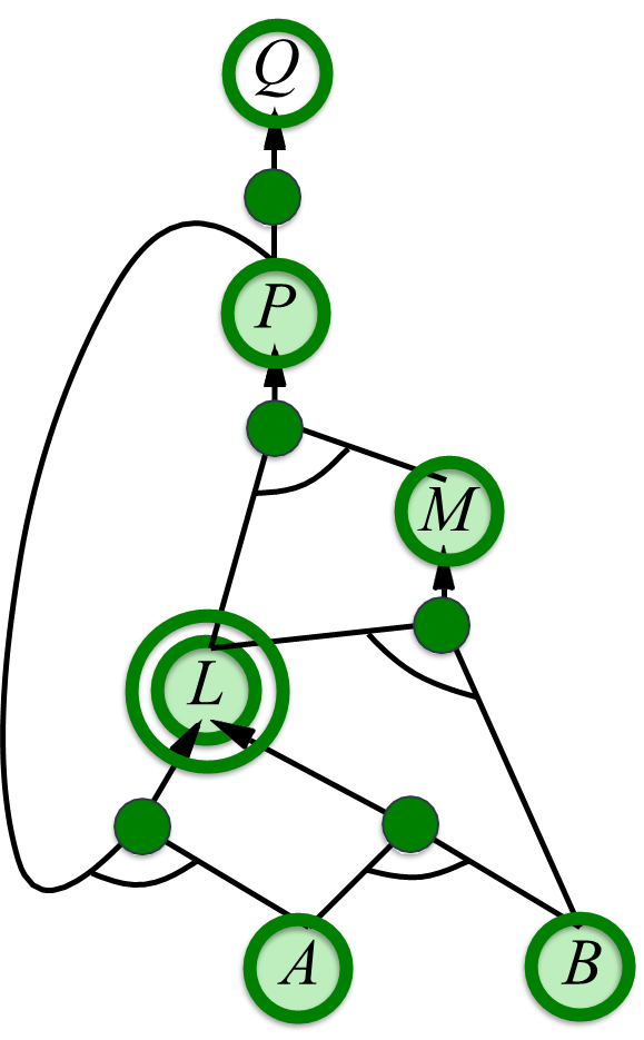
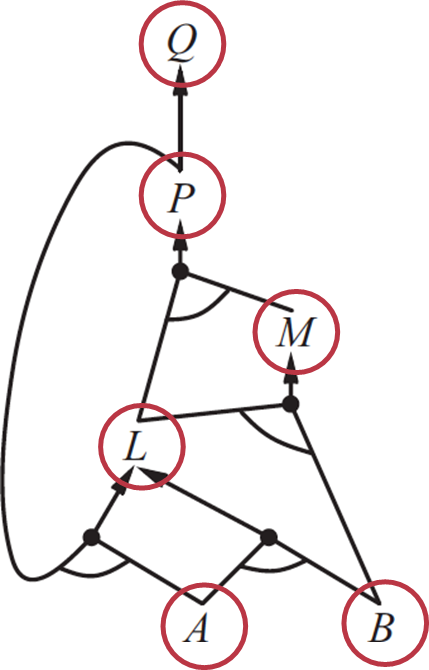
This recursive structure naturally maps onto an AND-OR graph, where links represent the premises of a single rule that must all be satisfied, and links represent the multiple alternative rules that could satisfy the same goal.
To ensure both computational efficiency and guaranteed termination, incorporates two crucial management checks:
Loop Detection: The algorithm must track the current path of goals (the goal stack) to detect and abandon paths where a subgoal attempts to prove itself through an ancestor goal (e.g., and ).
Memoization/Caching: Results for successfully proven or definitively failed subgoals are cached. If a subgoal is encountered again via a different path, its stored result is immediately retrieved, avoiding redundant, repeated work.
Example
Using the from the Forward Chaining example, we trace the goal-driven path to prove .
Goal : is the head of .
Subgoal:.
Goal : is the head of .
Subgoals:AND.
Subgoal : is the head of and (OR node). Try .
Subgoals:AND.
is Fact . (Proven).
is currently on the goal stack (). LOOP detected. is abandoned.
Subgoal (Revisit): Try .
Subgoals:AND.
is Fact . (Proven).
is Fact . (Proven).
Since and are proven, rule fires. L is proven. (Result cached).
Subgoal (Remaining from Step 2): is the head of .
Subgoals:AND.
is Fact . (Proven).
is retrieved from cache (Proven in Step 4).
Since and are proven, rule fires. M is proven.
Goal (Revisit from Step 2): Both subgoals and for rule are now proven.
Rule fires. P is proven.
Original Goal (Revisit from Step 1): The premise for rule is now proven.
Rule fires. Q is proven.
The goal-driven approach successfully traced the necessary chain of premises back to the initial facts, confirming the entailment.
Backward Chaining shares the high quality of inference associated with Forward Chaining, within the domain of definite clauses.
Soundness and Completeness: Backward Chaining is sound because, like Forward Chaining, it relies solely on the sound rule of Modus Ponens. It is also complete for definite clauses, guaranteeing that any positive literal entailed by the will be proven.
Computational Efficiency: For typical queries, is often more efficient than because it focuses the search only on rules that are logically relevant to the goal. In the worst case, however, can be slower if the goal is supported by a very deep and complex proof tree, although the use of caching prevents the exponential re-proving of subgoals.
The Difference: The key distinction is the direction of reasoning. is useful for constantly monitoring a changing environment and updating a set of beliefs (e.g., real-time diagnosis), while is optimal for finding the specific justification for a query and is the basis of many declarative systems (e.g., logic programming languages like Prolog).
A Logical Agent for the Wumpus World
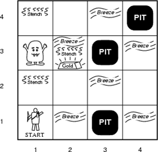
To understand how inference procedures are applied in practice, we can study a logical agent designed to operate in a simulated environment. The Wumpus World is a classic problem in artificial intelligence that serves as a testbed for reasoning and decision-making under uncertainty. It is a sufficiently complex environment to be interesting, yet simple enough to be modeled with propositional logic.
The world is a cave represented by a grid of rooms. The agent’s goal is to find a heap of gold and return to the starting square without being killed by the terrible Wumpus or falling into a bottomless pit.
To formally define the problem, we use the PEAS (Performance, Environment, Actuators, Sensors) framework.
Performance Measure:
for finding the gold and climbing out of the cave.
for falling into a pit or being eaten by the Wumpus.
for each action taken (to encourage efficiency).
for using the single arrow.
Environment:
A grid of rooms, with the agent always starting in square .
The locations of the Wumpus and the gold are chosen randomly in squares other than .
Each square (except ) can be a pit with a probability.
The environment is deterministic (actions have guaranteed outcomes), static (the Wumpus and pits do not move), discrete, and perceived by a single agent. It is also partially observable, as the agent only perceives its local surroundings.
Interaction:Grab (to pick up the gold), Shoot (fires the one arrow in a straight line), Climb (to exit the cave from ).
Sensors: The agent receives a percept from its current square:
Stench: In a square directly adjacent (not diagonally) to the Wumpus.
Breeze: In a square directly adjacent to a pit.
Glitter: In the square where the gold is.
Bump: If the agent walks into a wall.
Scream: Heard everywhere if the Wumpus is killed by the arrow.
A logical agent maintains a Knowledge Base (KB)—a set of sentences in a formal language that represents what it knows about the world. For the Wumpus World, we use propositional logic.
Propositional Symbols: We define symbols to represent facts about each square :
is true if there is a pit in square
is true if there is a breeze in square .
is true if the Wumpus is in square .
is true if there is a stench in square .
The Knowledge Base (KB):
The KB is composed of different types of knowledge:
Initial Knowledge: Facts true at the start. Since the agent begins in a safe square:
(No pit in )
(No Wumpus in )
Perceptual Knowledge: At each step, the agent adds sentences corresponding to its perceptions. At the start in , there is no breeze or stench:
Rules of the World (Atemporal Knowledge): These are rules that are always true. For example, a breeze in a square is equivalent to a pit in an adjacent square. For square , this is:
A complete KB would contain such a rule for every square in the grid.
The agent uses its KB and an inference procedure to deduce hidden properties of the world, such as which squares are safe to visit. A square is safe if .
Step 1: The Agent in Square [1,1]
The agent’s initial KB contains:
The agent wants to know if square is safe. It asks the query: ? To answer this, we use proof by refutation. We try to prove that is unsatisfiable. If it is, the original query holds. We use the DPLL algorithm for this.
DPLL Walkthrough to Prove : First, convert the KB and the negated query into Conjunctive Normal Form (CNF):
From (1):
From (2):
From (3), becomes three clauses:
The negated query to test for unsatisfiability is .
Our set of clauses is:
Step
Clause Set
Model
0
Init
1
Unit Propagation
2
Unit Propagation
3
Unit Propagation
4
Unit Propagation
5
Conflict
Conflict Found
Success
Conclusion: Since is unsatisfiable, we have proven that . By symmetry, the agent can also prove . The agent knows both adjacent squares are free of pits. Assuming it doesn’t smell a stench, it knows they are safe. It decides to move to .
Step 2: The Agent in Square [2,1]
The agent moves to and now perceives a Breeze. Its KB is updated:
All old knowledge is retained:, , , etc.
Newly derived knowledge is added:, .
New perceptual knowledge is added:.
New rules are now relevant:.
The agent now wants to assess the safety of its new neighbors, and . It asks the queries: ? and ?
Running DPLL on would find a satisfying model (e.g., one where is true, causing the breeze in , and is also true). Since it is satisfiable, the agent cannot prove that is free of pits. It is a possibly unsafe square. The same holds for .
A cautious agent will not enter a square that is possibly unsafe. The only provably safe action is to return to and then explore the other known safe square, , to gather more information. This process of iteratively gathering percepts, updating the KB, and making inferences allows the agent to safely navigate the world.
Limitations and Extensions
While effective for this simple scenario, using propositional logic this way has significant limitations.
Monotonicity: The KB only grows. Propositional logic is monotonic, meaning once a fact is added, it cannot be retracted. This is problematic for representing change over time.
Representational Burden: The KB becomes very large. We need a “breeze rule” and a “stench rule” for every single one of the 16 squares, leading to dozens of sentences.
The Problem of Time: Our model assumes a static world, but the agent’s position changes. We did not represent time in our propositions (e.g., ). To handle time, we need to introduce time-stamped propositions, known as fluents. For example, could mean the agent is at at time .
Introducing time leads directly to the Frame Problem: how to represent what doesn’t change after an action. If the agent moves from to , we need axioms stating that the Wumpus’s location, all pit locations, and the gold’s location remain unchanged. Writing these frame axioms for every action and every fluent is incredibly inefficient and scales poorly. A better solution involves using successor-state axioms, which describe for each fluent how it can become true or false, elegantly solving the frame problem. This, however, moves into a more expressive logical framework than simple propositional logic.
In our last step, the agent moved to the provably safe square . Upon arrival, it perceives a Breeze, but no Stench. The agent’s knowledge base is now expanded:
Initial KB: Contains all facts and rules from the start.
New Percept: (There is a breeze in ).
New Rule: The rule for breezes in is .
The agent now needs to assess the safety of the adjacent, unvisited squares: and . A square is safe only if it can be proven to contain neither a pit nor the Wumpus. Let’s focus on the pits and ask the query: ?
To solve this, we again use proof by refutation with the DPLL algorithm. We will test if the formula is satisfiable. If it is unsatisfiable, the query holds.
DPLL Walkthrough to Test : The set of clauses includes everything the agent knows plus the negation of our goal ().
Clauses:
From :
From :
Negated Conclusion:
Step
Clause Set
Model
0
Init
1
Unit Propagation
2
Unit Propagation
3
Unit Propagation
4
Unit Propagation
5
Unit Propagation
6
Unit Propagation
7
Final State
All clauses satisfied
Since we found a consistent set of assignments for all variables that makes all clauses in true, the formula is satisfiable.
Making a Safe Decision
The result of our inference is crucial:
Since is satisfiable, the agent cannot prove the conclusion .
This means that given what the agent knows, it is entirely possible for a pit to exist in square .
A cautious agent will not enter a square unless it is provably safe. Therefore, moving to is an unsafe action. By symmetry, the agent would also find that is satisfiable, meaning it cannot prove either.
The agent’s state of knowledge is that the breeze in must be caused by a pit in or (or both). Without more information, it cannot distinguish between these possibilities.
Success
The only provably safe action is to retreat. The agent should plan a path back to and then proceed to the other square it knows is safe: . By visiting and perceiving its surroundings, the agent can gather more information to further constrain the possible locations of pits and the Wumpus, hopefully proving the safety of other squares later on.
From Simple Inference to a Complete Logical Agent
The step-by-step reasoning process demonstrates the power of logical inference. However, this simplified model has major limitations when dealing with a changing world. To build a robust agent, we must address the challenge of representing time and its effects.
Time and Frame Problem
Our propositions like are atemporal—they do not have a time component. But the agent’s location, for instance, is not a permanent fact. To represent properties that change over time, we introduce fluents, which are propositions with a time index.
: The agent is at square at time .
: The agent has the arrow at time .
With fluents, we can write effect axioms that describe the outcome of actions. For example:
This states that being at and facing east at time 0, and then moving forward, results in being at at time 1.
This leads to a fundamental challenge known as the Frame Problem: How do we specify what remains the same after an action? The effect axiom above doesn’t say anything about the Wumpus’s location, the pit locations, or whether the agent still has the arrow. We would need to add a massive number of frame axioms for every action and every fluent, such as:
This approach is computationally infeasible due to the sheer volume of axioms required.
A more elegant solution is to change perspective. Instead of axioms for actions, we write one axiom for each fluent, describing all possible ways it could be true at the next time step (). This is a successor-state axiom, with the general form:
In words: A fluent is true at if either an action at made it true, OR it was already true at and no action at made it false.
Example
For example, the successor-state axiom for is very simple, as only one action can make it false:
This single axiom replaces numerous frame axioms and elegantly solves the representational frame problem.
The Qualification Problem
Even with a perfect model of change, another issue arises: the qualification problem. It is impossible to list all the preconditions for an action to succeed. For to work, the agent must be alive, not slipping, not being carried away by a giant bat, etc. Logic requires us to state all such conditions, which is impractical. In practice, agent designers list only the most important preconditions and ignore highly unlikely exceptions.
A Complete Hybrid Agent Architecture
By combining these concepts, we can define the architecture for a complete, albeit inefficient, logical agent.
The agent operates in a TELL-ASK cycle, formalized by the KB-AGENT function:
function KB-AGENT(percept) returns an action
  static: KB, a knowledge base
          t, a counter, initially 0

  TELL(KB, MAKE-PERCEPT-SENTENCE(percept, t))
  action ← ASK(KB, MAKE-ACTION-QUERY(t))
  TELL(KB, MAKE-ACTION-SENTENCE(action, t))
  t ← t + 1
  return action
TELL: The agent adds the new percept to its KB, using the time .
ASK: The agent queries the KB to determine the best action.
TELL: The agent records the chosen action in the KB.
A purely logical agent is often inefficient. A more practical design is a hybrid agent, which combines logical inference with other AI techniques:
Deduction: The agent uses its KB and successor-state axioms to deduce which squares are provably safe ().
Search/Planning: Once the safe squares are identified, the agent can use a search algorithm like A* to find the shortest path to an unvisited safe square or to the gold.
Finally, to overcome the performance degradation as increases, the agent employs logical state estimation. Instead of re-deriving the world state from its entire percept history, it maintains a belief state (the set of all possible current states of the world) and simply updates it with each new percept and action. This allows the agent to make decisions in constant time, independent of its history.