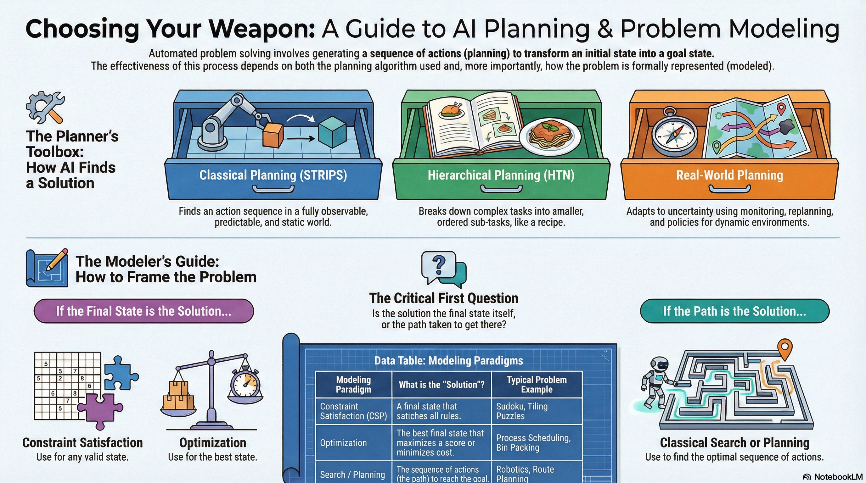
8.3 - Planning in Real World and Problem Modeling

Classical Planning and the STRIPS Formalism

Automated planning fundamentally addresses the computational challenge of determining an optimal or satisfactory sequence of actions that can systematically transform an initial, known configuration of the world into a predefined goal state. This paradigm, known as classical planning, operates under several strict assumptions: the environment is fully observable, deterministic (actions always have the same, predictable outcome), static (changes only occur due to the agent’s actions), and the agent has an explicit, complete model of the world. The complexity of solving such problems necessitates a formal, unambiguous language for representation, with the STRIPS (Stanford Research Institute Problem Solver) formalism being a cornerstone in Artificial Intelligence research.

The STRIPS Formalism

STRIPS, developed in the early 1970s, provides a simple yet powerful declarative language for describing planning problems.

Definition

A planning problem within the STRIPS framework is formally defined by a tuple , where is a set of propositions, is a set of operators (actions), is the initial state, and is the goal specification.

A key principle adopted by STRIPS is the Closed World Assumption (CWA), which posits that any proposition not explicitly stated as true in a given state is assumed to be false.

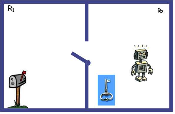
In the provided scenario involving a robot in a two-room environment (, ), the Initial State () is defined by a conjunction of positive ground literals (propositions without variables), representing all facts that are true at the start. Specifically, is given by

According to the CWA, the state implicitly contains the negation of all other possible propositions, such as or . The Goal State () is a partial specification—a conjunction of literals that must be satisfied for the problem to be solved: . Unlike the initial state, literals not mentioned in the goal are considered irrelevant; the plan is successful as long as all goal literals are true.

Action Schemas and State Transition

Actions, or operators, define the transitions between states. In STRIPS, an action schema specifies a Preconditions list (), an Add list (), and a Delete list (). The preconditions are a set of positive literals that must hold true in the current state for the action to be applicable. When an action is executed, all literals in its Delete-list are removed from the current state, and all literals in its Add-list are introduced, forming the resulting state. This structure effectively handles the Frame Problem—the issue of explicitly specifying which facts do not change—by only listing the changes ( and lists), and implicitly assuming everything else remains the same.

The provided action schemas illustrate this mechanism:

The action, where is a variable representing a room, requires the and to be in the same room (), deleting the predicate and adding the predicate.
The action requires and as preconditions, deleting and adding .
The action necessitates that the is in room , the is , and (the robot is moving to a distinct room). Executing it deletes and adds .

The entire planning task then reduces to searching the state-space graph, where nodes represent world states (conjunctions of true literals) and directed edges represent executable actions, seeking a path from the unique initial state to any state that satisfies the goal condition . The major difficulty in classical planning often lies in the exponential explosion of this state space, which is why efficient search algorithms and heuristic methods are critical to finding a valid plan.

Efficient Approaches to Classical Planning

While the foundational STRIPS formalism provides a structured representation for planning problems, the corresponding state-space graph can exhibit a combinatorial explosion, rendering basic classical search algorithms like Breadth-First Search (BFS) or A* search prohibitively inefficient for large domains. To overcome this limitation, more sophisticated and efficient techniques have been developed, primarily focusing on constraining the search space or leveraging problem structure. Key approaches include the SATPlan reduction, GraphPlan’s graph-based approach, and Hierarchical Planning’s use of abstraction.

SATPlan is a powerful method that strategically reframes the planning problem as a Boolean Satisfiability (SAT) problem. This involves generating a sequence of propositional formulas, , where each is satisfiable if and only if a plan of length exists. The formula incorporates representations of the initial state, the goal state at time , and an encoding of all action schemas and state transitions across time steps. By iteratively checking the satisfiability of using highly optimized SAT solvers, the shortest plan can be found. A satisfying assignment of the Boolean variables directly corresponds to a valid sequence of actions.

Hierarchical Planning (often formalized as Hierarchical Task Network - HTN planning) is inspired by human problem-solving, which often involves decomposition. This approach breaks down complex, high-level tasks into smaller, more manageable sub-problems, which are themselves recursively decomposed until they can be solved by primitive actions. This hierarchical structure significantly prunes the search space by focusing the planner on relevant sub-tasks, making it particularly effective for domains with inherent task structure.

GraphPlan

The GraphPlan algorithm, developed by Avrim Blum and Merrick Furst, offers a significant efficiency improvement by combining a forward, constructive approach with a backward, deductive search. It consists of two interleaved phases: graph expansion and solution extraction.

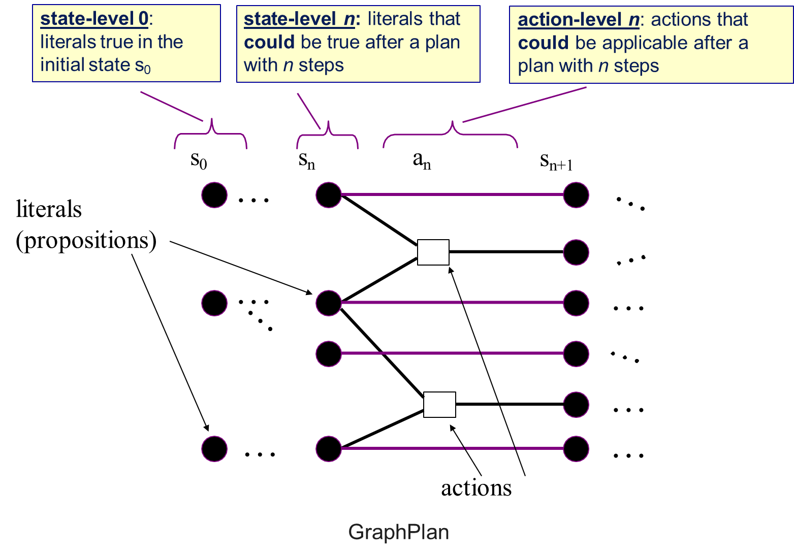
Phase 1: Planning Graph Expansion

The algorithm constructs a planning graph, which is a directed, bipartite graph alternating between State-Levels () and Action-Levels ().

State-Level (): Represents the set of all literals (positive or implicitly negative via CWA) that could potentially be true at time step .
Action-Level (): Represents the set of all actions whose preconditions are all present in the preceding state-level .

The construction proceeds iteratively from the initial state :

is initialized with the literals of the problem’s initial state .
is formed by identifying all actions from the operator set whose preconditions are subsets of the literals in . This level also includes persistence actions (or no-ops), which are meta-actions representing the fact that a literal from remains true in .
is formed by taking the union of the Add-lists of all actions and persistence actions in .

Example

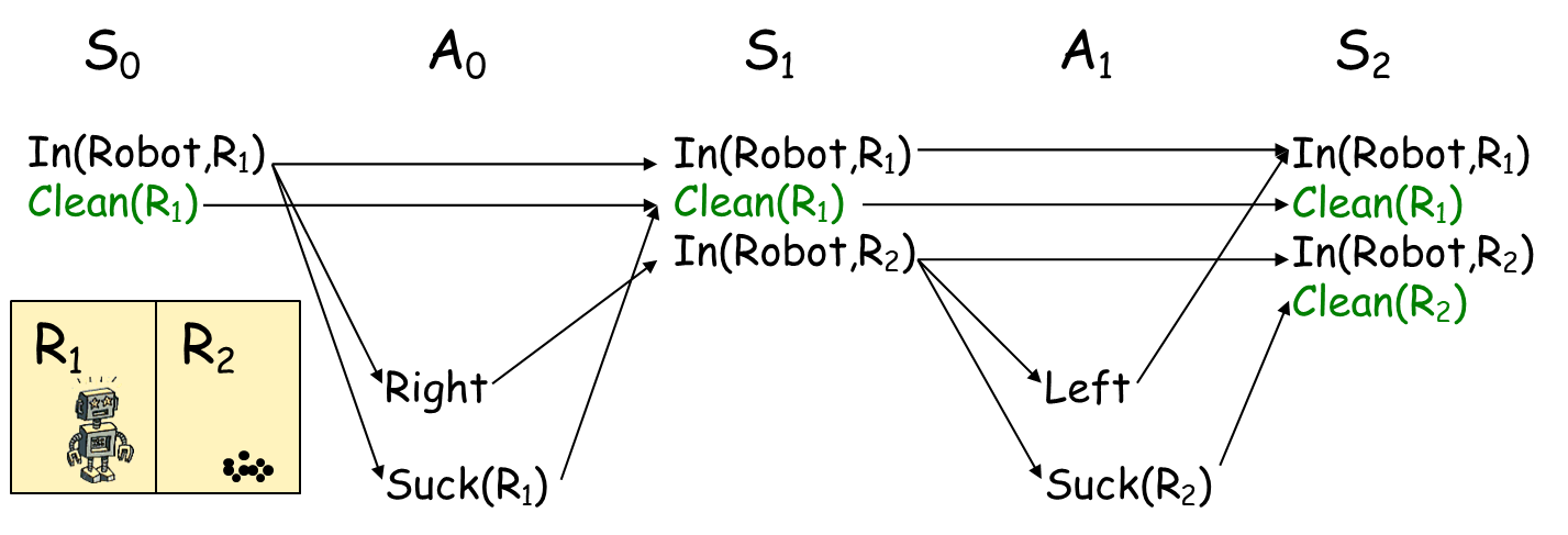
For the Vacuum-Cleaner World example, the graph expansion demonstrates this process:

includes (precondition ) and (precondition ), along with persistence actions for ‘s literals.

combines the Add-lists: adds , adds , and persistence maintains , leading to

The expansion continues until the graph levels off, meaning .

A critical concept for pruning the search space within the planning graph is mutual exclusion (mutex). Mutex links connect pairs of actions or literals that cannot co-occur in any valid plan at a given level.

Mutex Actions at : Two actions are mutex if one’s Add-list conflicts with the other’s Preconditions (destructive interference), if one’s Delete-list conflicts with the other’s Preconditions (inconsistent support), or if their Add-lists are in conflict (competing needs). For instance, the and actions may be mutex if deletes and requires it as a precondition.
Mutex Literals at : Two literals are mutex if all possible pairs of actions in that produce them are mutex. For example, and are mutex because they cannot be established simultaneously by non-mutex actions.

Phase 2: Solution Extraction

Once the goal literals are all present in and are pairwise non-mutex, the algorithm initiates a backward search from to find a valid plan. This search selects a non-mutex set of actions from that collectively satisfy all goal literals. The preconditions of these selected actions then become the subgoals for , and the process recurses until is reached. If the backward search fails, the graph is expanded to and the search is retried.

The index of the first state-level that contains the goal propositions, denoted as , is an effective heuristic known as the level cost. Since the graph construction makes no guarantees that the goal literals are non-mutex at this level, is an admissible heuristic (a lower bound on the true plan length) for the number of steps in the optimal plan. This makes it highly valuable for guiding external search algorithms like A*.

Hierarchical Planning and Task Network Decomposition

For problems of significant scale and complexity, particularly those found in robotics or game Artificial Intelligence (AI), the flat structure of classical planning with only primitive actions becomes computationally unmanageable and epistemologically inadequate. Hierarchical Planning addresses this challenge by introducing multiple levels of abstraction, formally realized through the Hierarchical Task Network (HTN) Planning paradigm. The HTN approach finds a plan by recursively decomposing abstract tasks until a sequence composed entirely of executable primitive actions is derived.

HTN planning defines a planning domain using three primary constructs, which allow for structured problem decomposition:

Primitive Tasks (Operators): These are the fundamental, executable actions that directly affect the world state, analogous to the STRIPS actions (e.g., ). They have explicitly defined preconditions and effects (Add and Delete lists).
Compound Tasks: Also known as abstract goals, these represent high-level objectives that cannot be executed directly (e.g., ). Achieving a compound task requires a structured decomposition process.
Methods (Decomposition Recipes): Methods specify how a particular compound task can be broken down into a partially ordered or totally ordered sequence of subtasks. A crucial feature is that a compound task may have multiple methods associated with it, each representing a distinct strategy for achieving the task.

The HTN planner’s objective is to search through the space of possible task decompositions, starting from an initial task network, until every node in the network is a primitive task. The final plan is the sequence of these primitive tasks in the resulting network. This contrasts sharply with classical state-space planning, where the search is conducted over world states. In HTN, the search is conducted over possible task networks.

Task Decomposition and Contextual Execution

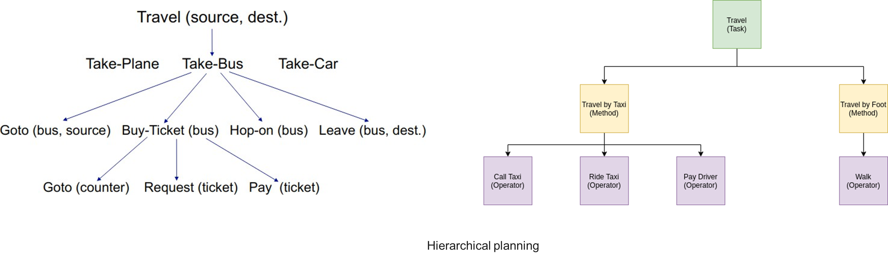
The Travel Planning example clearly illustrates the decomposition process. The compound task can be achieved by multiple high-level methods, such as , , or . The selection of a method depends on the prevailing constraints (e.g., distance, available resources). The chosen method, , then decomposes into a sequence of more specific subtasks: . Since is itself complex, it can be further decomposed into primitive actions like , , and , which are the actual executable steps.

The structured nature of HTN planning allows for highly context-aware and conditional behaviors, as highlighted by the game AI example involving the compound task .

Conditional Methods: Methods often include conditions that must be satisfied for the decomposition to be applicable. The first method, , is only chosen if the agent’s world state () indicates an enemy is visible. This path leads to the execution of subtasks: .
Default/Fallback Methods: The second method, , is a default choice, applicable when the primary condition is false. This decomposition, , guides the agent to a different, less aggressive behavior when no immediate threat is present.

Compound Task [BeTrunkThumper] 
	Method [WsCanSeeEnemy==true] 
		Subtasks [NavigateToEnemy(), DoTrunkSlam()] 
	Method [true] 
		Subtasks [ChooseBridgeToCheck(), NavigateToBridge(), CheckBridge()]

Primitive Task [DoTrunkSlam] 
	Operator [AnimatedAttackOperator(TrunkSlamAnimNa 
	
Primitive Task [NavigateToEnemy] 
	Operator [NavigateToOperator(EnemyLocRef)] 
		Effects [WsLocation = EnemyLocRef] 
	
Primitive Task [ChooseBridgeToCheck] 
	Operator [ChooseBridgeToCheckOperator] 

Primitive Task [NavigateToBridge] 
	Operator [NavigateToOperator(NextBridgeLocRef)] 
		Effects [WsLocation = NextBridgeLocRef] 

Primitive Task [CheckBridge] 
	Operator [CheckBridgeOperator(SearchAnimName)]

This ability to incorporate conditional logic and structural constraints directly into the decomposition recipes is what grants HTN planning its power in generating plans that reflect complex, domain-specific strategies, moving beyond the simple goal-reaching of basic STRIPS. The execution of the Primitive Task , for instance, is directly linked to an Operator that, upon completion, enforces a change in the world state, such as setting the agent’s location to the enemy’s location (). HTN planning systems are thus particularly well-suited for systems where the path to the goal is more important than just the final state (e.g., following a specific protocol or procedure).

Real-World Planning and Robustness

While formalisms like STRIPS and algorithms like GraphPlan provide a rigorous foundation for automated reasoning, they operate within a theoretical vacuum defined by strict, often unrealistic constraints. Deploying planning agents in the real world necessitates a departure from these idealized conditions.

The Limitations of Classical Assumptions

Classical planning rests upon a “closed-world” philosophy, assuming a controlled environment where the agent is effectively omniscient and omnipotent within its domain. Specifically, these algorithms presume:

the environment is fully observable (the agent has perfect, zero-latency access to the global state) and deterministic (actions obey strict physical laws with unique, predictable outcomes).
the world is assumed to be static and discrete; strictly speaking, this means no changes occur unless initiated by the agent (no “exogenous events”), and time and space can be cleanly divided into distinct steps or grid units.

Classical planning typically assumes a single-agent context where the planner is the sole active entity, operating with a complete and correct model of the “laws of physics” governing the domain.

In reality, these assumptions rarely hold: sensors are noisy and limited (partial observability), motors slip and fail (stochasticity/non-determinism), and environments are dynamic, populated by other actors or natural forces that change the state of the world independently of the agent. When these assumptions are violated, a classical plan—which is essentially a rigid, linear script—becomes brittle and prone to catastrophic failure.

Uncertainty and Multi-Agent Systems

To address these limitations, the planning paradigm must be extended to incorporate uncertainty and external interaction.

Non-Deterministic and Sensorless Planning

When the assumption of determinism is relaxed, an action may result in one of several possible outcomes. If the agent also lacks sensory feedback—a scenario known as Sensorless Planning—it faces a profound challenge. In this context, the agent does not track a single current state but rather a belief state, which is the set of all physical states the world might be in.

The objective is to find a conformant plan: a sequence of actions that coerces the world into the goal state regardless of which non-deterministic outcomes actually occur.

Conditional Planning and Policies

When the environment is partially observable but the agent possesses sensors, it can employ Conditional Planning (or Contingency Planning). Unlike classical plans, which are linear sequences, conditional plans introduce branching logic. The planner generates a structure that resembles a decision tree, incorporating sensing actions to disambiguate the state of the world at runtime.

The output is often not a fixed plan, but a policy ().

Definition

A policy is a mapping from every possible perceived state (or belief state) to an optimal action ().

For instance, a rover on Mars might have a policy: “Approach rock. IF spectrometer indicates carbonates, drill. ELSE, move to next target.” This allows the agent to react adaptively to information that is only available during execution.

Multi-Agent Planning (MAP)

The Multi-Agent Planning extension relaxes the single-agent assumption, acknowledging that the environment is populated by other autonomous entities. This introduces significant complexity because the environment becomes non-static; changes occur due to the actions of others. MAP distinguishes between cooperative environments (e.g., a swarm of drones fighting a fire), where agents share a joint goal and must coordinate to avoid collisions or redundancy, and adversarial environments (e.g., chess or military strategy), where agents must model the opponent’s intentions to optimize their own utility.

Execution Monitoring and Dynamic Replanning

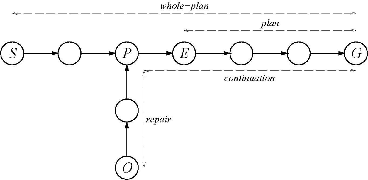
Given that real-world models are rarely perfect, an agent must be capable of Execution Monitoring. This involves a continuous control loop: Planning Execution Observation. The agent constantly compares its percepts (the actual state, ) against its internal prediction (the expected state, ). If a discrepancy is detected—indicating the plan has failed—the agent must initiate a Replanning phase.

We can categorize replanning strategies based on how they handle the deviation from the expected path. Consider a scenario where an agent intended to move from a pre-failure state to an expected state , but an unexpected event places it in state .

Global Replanning (Plan to ): The most robust but computationally expensive approach. The agent discards the existing plan entirely and invokes the planner to find a new path from the current actual state to the ultimate goal .
Plan Repair (Plan to ): The agent attempts to minimize computational effort by “fixing” the local error. It searches for a short sequence of actions to return from the deviant state back to the pre-failure state (or the original expected state ), effectively trying to get “back on track” to resume the original plan.
Serendipitous Replanning: Occasionally, an unexpected event may be beneficial. If the state is actually closer to the goal than was, the agent can exploit this “luck” by planning a new, shorter path from to a later stage in the original plan, bypassing intermediate steps.

In highly dynamic environments where the world changes faster than a complete plan can be generated, agents may adopt an Online Planning strategy. Rather than formulating a complete solution from start to finish, the agent plans only a short “horizon” into the future (e.g., the next 5 steps), executes the first step, observes the result, and immediately replans the updated horizon. This “look-ahead” approach allows the agent to remain responsive to a rapidly changing environment.

Problem Modeling

Before any computational algorithm can be successfully applied, the problem at hand must be translated into a formal model. This phase is arguably the most critical step in the engineering process, as the choice of representation—how states, actions, and goals are defined—directly dictates the computational complexity and the specific family of algorithms suitable for finding a solution. An ill-conceived model can render a trivial problem intractable, while an elegant model can expose efficient heuristics and solution paths.

Framework for Problem Classification

To select the appropriate algorithmic approach, one must first fundamentally categorize the nature of the problem. This categorization hinges on the definition of a “solution” within the specific domain.

Path-Based vs. State-Based Solutions

The primary distinction lies in whether the solution is defined by the state itself or the path taken to reach it. In problems such as route planning, logistics, or the 8-puzzle, the final state is often trivial or explicitly known (e.g., “be at the destination”); the computational challenge is to discover a valid sequence of actions (a path) that transitions the system from an initial state to the goal state.

These problems fall under the domain of Classical Search or Automated Planning. Conversely, in problems like the N-queens puzzle, Sudoku, or exam scheduling, the sequence of steps taken to arrange the elements is irrelevant. The objective is simply to find a specific configuration (state) that satisfies a set of constraints. These are classified as Constraint Satisfaction Problems (CSPs) or optimization problems, where the cost or utility is associated with the state itself (e.g., the number of constraint violations) rather than the transition cost.

Cost Dynamics in Path-Finding

Within path-based problems, a further distinction must be made regarding the cost of actions. If the objective is to optimize the journey—finding the path with the lowest cumulative cost—algorithms that account for edge weights, such as A* or Uniform Cost Search, are required. These algorithms utilize an objective function to minimize the path cost, . However, if all actions are effectively equal (having a uniform cost, typically 1) and the goal is simply to find the shortest path in terms of the number of steps, unweighted search strategies like Breadth-First Search (BFS), Depth-First Search (DFS), or Iterative Deepening Search (IDS) are sufficient and often more computationally efficient.

Choosing a State Representation

The efficiency of a solver is heavily influenced by the “structure” or level of abstraction used to represent the world states. There are three primary levels of state representation, offering a trade-off between expressiveness and algorithmic complexity.

Atomic Representations

At the lowest level of complexity is the atomic representation, where each state is treated as a “black box” with no internal structure. In this model, states are indivisible entities (e.g., node “A” or node “B” in a graph). The algorithm can check for equality (is State A the same as State B?) but cannot reason about why a state is desirable or how close it is to a goal based on its features. This representation is standard for basic graph search algorithms like BFS or DFS but is limited in its ability to support complex heuristics.

Factored Representations

A significant leap in expressiveness is achieved with factored representations. Here, a state is defined by a fixed set of variables or attributes, each assigned a value.

For example, a state might be represented as a vector . In a map-coloring problem, a state is not just a node, but a collection of variable-value pairs (e.g., ).

This allows algorithms to examine the internal components of a state, enabling the development of heuristics based on the number of satisfied variables, which is essential for CSPs and local search algorithms.

Structured Representations

The most expressive form is the structured representation, which models the world using objects and the logical relationships between them, often utilizing a subset of First-Order Logic. A state is described by a conjunction of literals, such as . Unlike factored representations, which typically have a fixed number of variables, structured representations can describe worlds with varying numbers of objects and complex, relational dynamics. This is the standard for Classical Planning (using languages like STRIPS or PDDL), as it allows the solver to reason about general rules (actions) that apply to classes of objects.

Practical Guidelines for Modeling

To synthesize these concepts into a practical workflow, one can apply a decision-making hierarchy when approaching a new problem.

If the problem requires a sequence of actions to transition between states, it should be modeled as a search problem. If the internal structure of the state is relevant to the transitions (as in robotics), a Planning approach using structured states is ideal; otherwise, Classical Search with atomic or factored states suffices.

If the sequence is irrelevant and the goal is merely to find a specific configuration, the choice depends on the nature of the goal states. If some final states are “better” than others (e.g., minimizing fuel consumption or maximizing schedule preferences), the problem should be modeled as an Optimization problem, solvable via Local Search techniques like Hill Climbing or Simulated Annealing. However, if all valid final states are equally acceptable—meaning the difficulty lies solely in finding any state that satisfies the rules—the problem is best modeled as a Constraint Satisfaction Problem (CSP).

Case Studies

Case Study 1: The Sliding Tile Puzzle

To solidify the principles of problem modeling, we will now analyze a classic AI problem: a variation of the sliding tile puzzle. This case study demonstrates how the same underlying problem can be framed as a classical search problem or a planning problem, depending on the chosen representation.

The puzzle consists of a linear board with seven slots. Initially, the board is configured with three black tiles (B), three white tiles (W), and one empty space, as follows:

The goal is to reach a configuration where all white tiles are to the left of all black tiles. The final position of the empty space is irrelevant.

There are two types of moves available, each with an associated cost:

Slide: A tile can move into an adjacent empty location. This action has a cost of 1.

Jump: A tile can jump over one or two other tiles into the empty location. The cost is equal to the number of tiles jumped over (i.e., cost of 1 for 1 tile, cost of 2 for 2 tiles).

We define the search problem components using a factored or atomic state representation.

States: A state is a permutation of the 7 slots. We can represent this as a tuple of length 7: , where each slot can be in one of the three possible states: .

Initial State ():

Actions(s): The set of actions available in a given state . The actions are defined by the legal moves. To be systematic, we can restrict the movement of tiles: black tiles can only move rightward, and white tiles can only move leftward. This is a common heuristic constraint to prevent cycles and reduce the branching factor.

For each black tile at position :

Slide: If position is empty, an action move(x, x+1) is available with cost 1.

Jump 1: If is occupied and is empty, an action move(x, x+2) is available with cost 1.

Jump 2: If and are occupied and is empty, an action move(x, x+3) is available with cost 2.

For each white tile at position :

Similar rules apply for leftward movement (e.g., move(x, x-1), move(x, x-2), etc.).

Transition Model (): This function returns the new state resulting from executing action . For example, executing jump(2, 4) (indices 1-based) on results in:

Goal Test: A function that checks if all ‘W’s precede all ‘B’s. A sample goal state is .

Step Costs: The cost of each action is defined by the move type (1 for a slide or 1-tile jump, 2 for a 2-tile jump). Since the problem involves finding a sequence of moves (a path) and the actions have non-uniform costs, an algorithm like A* Search or Uniform Cost Search would be appropriate to find the optimal solution.

Modeling as a Planning Problem

We now reformulate the problem using the structured representation of classical planning (STRIPS/PDDL).

Predicates and Constants:

Constants:

: Represent the locations on the board.

: Represent the colors of the tiles.

Predicates (Propositions):

: A tile of color is at location . (e.g., )

: Location is empty. (Note: This can also be represented implicitly by the absence of an predicate for that location).

$₁ ₂$ : Location $₁$ is adjacent to location $₂$ . This is a static predicate, true for pairs like , , etc.

Initial State: A conjunction of ground literals defining the board layout and tile positions:

$You can't use 'macro parameter character #' in math mode \begin{aligned} I = &\bigwedge_{i=1}^{6} ADJ(i, i+1) \land \bigwedge_{i=1}^{6} ADJ(i+1, i) \land \\ & AT(B,1) \land AT(B,2) \land AT(B,3) \land \\ & Empty(4) \land \\ & AT(W,5) \land AT(W,6) \land AT(W,7) \end{aligned} $$ In this formulation, $AT$ and $Empty$ are **fluents** because their truth value changes as actions are performed. $ADJ$ is **static** because the board's layout never changes. 3. **Goal State**: The goal is a logical expression that must be satisfied. Assuming we have a greater-than predicate $>$ defined over locations, the goal can be stated as: $$∀ l_{1}, l_{2}, c_{1}, c_{2}, (AT(c_{1},l_{1}) ∧ c_{1}=W ∧ AT(c_{2},l_{2}) ∧ c_{2}=B) \implies l_{2} > l_{1}$$ In a simpler, grounded form for this specific problem instance: $$ \begin{aligned} AT(W,u) ∧ AT(W,v) ∧ AT(W,w) ∧ AT(B,x) ∧ AT(B,y) ∧ AT(B,z) ∧\\ x>u ∧ x>v ∧ x>w ∧ y>u ∧ y>v ∧ y>w ∧ z>u ∧ z>v ∧ z>w \end{aligned} $$ 4. **Action Schemas**: Action schemas are templates for actions. Here are schemas for the "slide" and "jump" moves: * **Schema: `MoveToEmpty(t, from, to)`** (Slide an adjacent tile $t$ from $from$ to $to$) * **Preconditions (P):** $AT(t, from) ∧ Empty(to) ∧ ADJ(from, to)$ * **Effects (E):** $AT(t, to) ∧ Empty(from) ∧ ¬AT(t, from) ∧ ¬Empty(to)$ * **Schema: `JumpOne(t, from, over, to)`** (Jump tile $t$ from $from$ over location $over$ to $to$) * **Preconditions (P):** $AT(t, from) ∧ Empty(to) ∧ ADJ(from, over) ∧ ADJ(over, to)$ * **Effects (E):** $AT(t, to) ∧ Empty(from) ∧ ¬AT(t, from) ∧ ¬Empty(to)$ * **Schema: `JumpTwo(...)`** can be defined similarly. "*Are black tiles forced to move rightward and white tiles leftward?*" Not with these general schemas. The `MoveToEmpty` action schema allows a black tile at location 3 to move left to an empty location 2, which is undesirable. To enforce directional movement, the preconditions would need to be more specific, for example by adding $color(t)=B ∧ from < to$ to the precondition list for black tile moves. ### GraphPlan Simulation (Step 1) Let's trace the first expansion of the planning graph for this problem. - **$S_0$ (State Level 0):** Contains the initial literals: $$\{ AT(B,1), AT(B,2), AT(B,3), Empty(4), AT(W,5), AT(W,6), AT(W,7) \}$$ - **$A_0$ (Action Level 0):** The planner identifies all actions satisfied by $S_0$. - `MoveToEmpty(B, 3, 4)`: Slide B from 3 to 4. - `JumpOne(B, 2, 3, 4)`: Jump B from 2 to 4. - `JumpTwo(B, 1, 2, 3, 4)`: Jump B from 1 to 4. - `MoveToEmpty(W, 5, 4)`: Slide W from 5 to 4. - (plus symmetrical moves for W and all persistence actions). - **$S_1$ (State Level 1):** The union of Add-lists from $A_0$. - $S_1$ now contains literals like $AT(B,4)$ and $AT(W,4)$. Note that these are **mutually exclusive** in this level (mutex), as they cannot both be true simultaneously in a valid single world state, but they both exist as _possibilities_ in the planning graph. ### Comparison of Models | Feature | Search Problem Model | Planning Problem Model | | :--- | :--- | :--- | | **State Representation** | **Factored/Atomic:** A single data structure (e.g., an array) represents the entire board. It's holistic and less descriptive. | **Structured:** A set of logical propositions describing objects and their relationships. It's compositional and more expressive. | | **Action Representation** | **Procedural Code:** Actions are functions that transform one state object into another. (e.g., `def move(state, from, to): ...`) | **Declarative Schemas:** Actions are described by their preconditions and effects. The planner's inference engine handles the state transformation. | | **Domain Knowledge** | Often encoded implicitly within the action functions or heuristics. | Can be expressed explicitly and declaratively through predicates and axioms. | | **Solution Method** | Graph search algorithms like A\*. | Domain-independent planners like GraphPlan or SATPlan. | | **Flexibility** | Less flexible. Changing the rules (e.g., adding a new type of move) requires rewriting the action functions. | More flexible. Changing rules often means just adding or modifying action schemas, without changing the planner itself. | Both models are valid, but the planning approach separates the **domain logic** (the rules of the puzzle) from the **solution logic** (the algorithm), making it more robust to changes in the problem definition.$

Case Study 2 - The Food Buying Problem

This case study transitions the analytical focus from pathfinding algorithms to combinatorial optimization. Unlike navigation problems where the objective is to determine a specific sequence of actions to reach a destination, the “Food Buying Problem” necessitates identifying a final configuration—specifically, a combination of items—that maximizes a utility function while adhering to strict resource constraints.

The core objective is to determine the optimal subset of food items that can be purchased within a fixed budget of 300 yen. Optimality is defined by maximizing the aggregate satisfaction score of the selected items. The problem imposes two critical constraints: the cumulative price of the selected items must not exceed the budget, and no single item type may be selected more than twice.

This scenario represents a variation of the classic Knapsack Problem, a fundamental problem in combinatorial optimization. Specifically, because the problem allows for the selection of multiple copies of an item (up to a limit of two), it is formally classified as the Bounded Knapsack Problem (BKP).

Mathematically, let be the set of available item types, where each item has a cost and a satisfaction score (value) . Let be the quantity of item selected. The optimization objective is to:

Subject to the constraints:

Budget Constraint:

Quantity Constraint: for all

The available items include Cake Slices, Macarons, Chocolate Slices, Cookies, Soda, and Water, each possessing distinct price-to-utility ratios.

Item Image Score Price (yen)
Cake Slice 🍰 5 105
Macarons 🍪 7 170
Chocolate Slice 🍫 10 180
Cookies 🍪🍪 3 50
Soda 🥤 4 130
Water 💧 6 130

Modeling as an Optimization Problem (Local Search)

This problem is naturally suited for an optimization framework utilizing local search algorithms. In this model, the algorithm operates on a complete state formulation rather than building a solution incrementally.

State Representation and Constraints

A state is defined as a multiset of food items. To constitute a valid or “legal” state, the multiset must satisfy the problem’s constraints.

Example

a state containing is legal because the total cost (50 + 50 + 130 = 230 yen) is within the budget and no item count exceeds two.

a state such as is illegal because the aggregate cost (180 + 105 + 105 = 390 yen) violates the budget constraint, rendering it an invalid candidate solution.

Objective Function

The utility or objective function assesses the quality of a state. In this context, the function calculates the summation of the satisfaction scores of all items currently in the set. The goal of the local search algorithm is to navigate the state space to discover the state with the highest global maximum utility.

Example

For the state , the utility is .

For the state , the utility is .

Local Moves and the State Space Landscape

Local search algorithms explore the state space by transitioning from the current state to a “neighboring” state via local moves. Standard operators include adding a new item to the set or substituting an existing item with a different one. However, a critical consideration in local search design is the inclusion of a “remove item” operator.

While counterintuitive to the goal of maximizing a score, the ability to remove an item is essential for navigating the state space landscape, particularly for escaping local maxima. A local maximum is a state that is better than all its immediate neighbors but inferior to the global optimum.

(Cost: 300, Score: 13). Any attempt to add or substitute items might violate the budget constraint. Without a "remove" operator, the algorithm would be trapped. By allowing the removal of an item (e.g., removing Water), the algorithm temporarily reduces the score but frees up budget, potentially opening a path toward a globally optimal state like (Score: 16).

For instance, an algorithm might reach a state

Modeling as a Search Problem

Although less intuitive than the optimization model, this problem can be framed as a constructive search problem, similar to pathfinding. Here, the “path” represents the sequence of purchasing decisions, and the solution is built step-by-step.

State Space and Transitions

The initial state is represented by an empty basket (), a current cost of zero, and a set of available items . To strictly enforce the “at most twice” constraint within the search structure, the set must contain unique identifiers for each instance of an item (e.g., ).

The transition model involves an action “add item ,” which is valid only if adding the item does not exceed the budget. Applying this action on the state results in a new state .

The goal state is reached when no further items can be added from without violating the budget constraint.

Step Cost Transformation

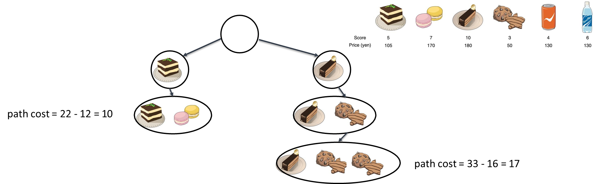
The most complex aspect of this model is the definition of step cost. Standard search algorithms like Uniform Cost Search or A* are designed to minimize path cost, whereas this problem requires maximizing utility. Therefore, the utility function must be inverted or transformed into a cost function.

Several transformation strategies exist to align the maximization objective with minimization algorithms:

Inverse Score (): Assuming a maximum possible item score of 10, one can define the cost of adding an item as minus its score. Consequently, items with high utility incur a low path cost, encouraging the search algorithm to select them.

Reciprocal Score (): Alternatively, defining the cost as the reciprocal of the score ensures that high-value items add only a small fractional cost to the path, making them preferable.

Negative Utility: One could define the step cost as the negative value of the score. However, many standard search implementations assume non-negative step costs, making the previous two transformations more robust for general-purpose algorithms.

Modeling as a Planning Problem

The Food Buying Problem can also be represented using automated planning formalisms, though this approach poses significant challenges due to the arithmetic nature of the constraints.

Classical planning (e.g., using basic STRIPS) relies on logical predicates. Modeling this problem requires defining predicates such as for items in the basket and for available items. In this way, the initial state includes all items as (), and the goal state requires maximizing the number of items while respecting the budget. However, standard classical planners are designed for satisficing—finding any sequence of actions that leads to a goal state—rather than optimizing for a numerical value.

To effectively model the budget and utility maximization, one must utilize more expressive planning languages, such as PDDL (Planning Domain Definition Language) with specific extensions.

Numeric Fluents: The problem requires arithmetic operations to track the cumulative cost. An action schema for Select(item) would require preconditions checking if current_cost + item_cost <= 300 and effects that update the current_cost.

Plan Metrics: To address the maximization goal, the planner must support metrics (e.g., (:metric maximize (total-score))). Without this extension, a planner might return a valid plan that simply fills the basket with low-value items, satisfying the constraints but failing the optimization objective.

Therefore, while a planning model is theoretically possible, the Optimization/Local Search model remains the most direct and computationally efficient representation for this specific Bounded Knapsack variation.

Item	Image	Score	Price (yen)
Cake Slice	🍰	5	105
Macarons	🍪	7	170
Chocolate Slice	🍫	10	180
Cookies	🍪🍪	3	50
Soda	🥤	4	130
Water	💧	6	130

Case Study 3 - Tiling with Dominoes
The third case study transitions from numeric optimization to combinatorial geometry and constraint satisfaction. The “Tiling with Dominoes” problem represents a class of problems where the objective is not to maximize a value or find a shortest path, but rather to determine the existence of a valid configuration that strictly adheres to a set of binary constraints.

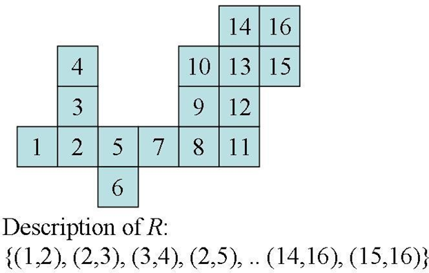
The problem asks whether a specific planar region , composed of unit squares, can be perfectly tiled by dominoes. A domino is defined geometrically as a rectangle, capable of covering exactly two adjacent unit squares within the grid.

Mathematically, this problem is equivalent to finding a perfect matching in a graph. If we construct a graph where each vertex represents a square in region , and an edge exists if and only if squares and are adjacent, then a valid tiling corresponds to a set of disjoint edges that cover every vertex in the graph.

The solution must satisfy three fundamental constraints:

Geometry: Each domino must cover exactly two adjacent squares (edges in the graph).

Completeness (Surjectivity): Every square in the region must be covered.

Exclusivity (Injectivity): No two dominoes may overlap; that is, no square may be covered by more than one domino.

Modeling as a Constraint Satisfaction Problem (CSP)

Constraint Satisfaction Problems (CSPs) are mathematically defined by a set of variables, a domain of values for each variable, and a set of constraints restricting the allowable combinations of values. This tiling problem offers two distinct CSP formulations, which illustrate the importance of variable selection in algorithmic efficiency.

Model 1: Domino-Centric Formulation

In this model, the variables represent the physical dominoes themselves, denoted as . The domain for each variable consists of all valid positions on the board—specifically, all sets of coordinate pairs representing adjacent squares in .

For example, a suitable domain value for domino could be , representing all possible placements of that domino on the grid.

The primary constraint is that of non-overlap, often formalized as an AllDiff constraint, ensuring that for all .

However, this model suffers from a critical deficiency regarding the completeness constraint. While the formulation prevents overlaps, it does not inherently guarantee that the union of all domino placements covers the entire region (). Enforcing this requires a complex global constraint checking that every coordinate in appears in the assignment set. This lack of constraint propagation makes the model computationally inefficient and difficult to implement using standard solvers.

Model 2: Square-Centric Formulation (Dual Model)

A superior approach involves inverting the perspective so that the squares themselves are the variables . The domain of a variable is the set of potential domino placements that could cover that specific square. For example, square 1 could be covered by a domino placed either horizontally (covering squares 1 and 2), while square 2 could be covered by a domino placed either horizontally (covering squares 1, 2 and 3) or vertically (covering squares 2 and 5).

The constraints in this model enforce consistency between adjacent variables. If variable is assigned the value corresponding to a domino covering squares and (denoted as ), then the variable must necessarily be assigned the same value . This formulation is powerful because it relies on local constraints between neighbors. This structure allows constraint propagation algorithms, such as AC-3 (Arc Consistency Algorithm #3), to rapidly prune the search space. If a decision is made for one square, the implications immediately propagate to its neighbors, drastically reducing the branching factor and ensuring that both completeness and exclusivity are inherently satisfied.

Modeling as an Optimization Problem

While less conventional for exact tiling, the problem can be framed as an optimization task suitable for Local Search algorithms like Hill Climbing. In this context, a state is defined as a configuration of dominoes placed on the board, potentially including invalid placements (overlaps or gaps).

The search landscape is defined by a cost function (or energy function) that quantifies the “badness” of a state. A robust objective function would be the sum of constraint violations:

The algorithm aims to minimize this cost to zero.

Local moves (transitions) involve modifying the current configuration. A typical operator might select a domino and attempt to rotate it around one of its constituent squares (e.g., moving a domino covering and to cover and ). A significant challenge with this approach is the high prevalence of local minima.

Tiling problems are often “fragile,” meaning a correct solution requires a specific global arrangement, and local greedy moves often lead to dead ends where no single rotation can reduce the error, necessitating random restarts or simulated annealing to escape.

Modeling as a Search or Planning Problem

The problem can be modeled as a sequential decision process, though this is often less efficient than the CSP approach due to the state-space explosion.

The initial state is an empty board.

The action space consists of placing a single domino on any pair of adjacent, unoccupied squares.

The transition model returns a new board state with the domino added.

The goal test checks if the number of covered squares equals .

If one were to apply BFS to this model, the algorithm would initialize a queue with the empty board. In the first iteration, it would generate successors for every possible valid placement of the first domino. For a large grid, this results in a massive branching factor immediately. The algorithm then explores placing a second domino for every one of those branches. This combinatorial explosion makes uninformed search impractical for all but the smallest regions.

Using a formalism like STRIPS or PDDL, the problem utilizes predicates such as , , and .
Predicates: 
            Covered(s), 
            Uncovered(s), 
            Placed(d), 
            Unplaced(d)
Constants: 
            Squares: {s1, s2, ..., s2n} 
            Dominoes: {d1, d2, ..., dn}
Initial State: 
            Uncovered(s_1) ∧ Uncovered(s_2) ∧ ... ∧ Uncovered(s_2n) ∧
            Unplaced(d_1) ∧ Unplaced(d_2) ∧ ...∧ Unplaced(d_n)
Goal State: 
            ∀ s_i, Covered(s_i)
Action Schema: 
            PlaceDomino(d, s_a, s_b)
Preconditions: 
            Unplaced(d) ∧ Uncovered(s_a) ∧ Uncovered(s_b) ∧ Adjacent(s_a, s_b)
Effects: 
            ¬Uncovered(s_a) ∧ ¬Uncovered(s_b) ∧ ¬Unplaced(d) ∧ Covered(s_a) ∧ Covered(s_b) ∧ Placed(d)
While logically sound, this planning model faces the same efficiency hurdles as the constructive search. Without domain-specific heuristics to guide the planner (e.g., “always tile corners first” or “prioritize squares with fewest remaining neighbors”), a general-purpose planner will struggle to find a solution in the vast search space. Thus, the CSP formulation remains the standard academic approach for solving such tiling problems.

Case Study 4 - Process Scheduling

The fourth case study examines a fundamental challenge in computer science and operations research: Process Scheduling.

The objective of the Process Scheduling problem is to allocate a set of computational tasks, distinctively termed “processes,” to a set of available hardware resources, or “computers.” The goal is not merely to find a valid assignment but to identify an optimal configuration that minimizes the total number of occupied computers. This efficiency is critical in real-world scenarios, such as cloud computing or data center management, where reducing active hardware leads to energy savings and lower operational costs.

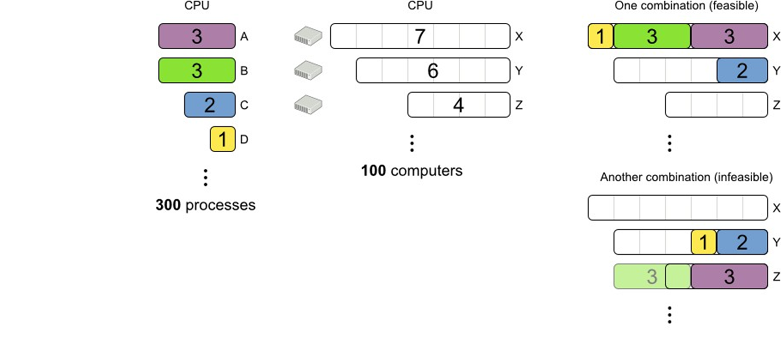
Formally, the problem involves a set of 300 processes and 100 computers. Each entity possesses specific numerical attributes: processes have a “size” (representing memory or CPU requirements), and computers have a “capacity” (the maximum total size they can accommodate). The governing constraint is a strict capacity limit: the sum of the sizes of all processes assigned to a specific computer must not exceed that computer’s capacity.

This scenario is a classic instance of the Bin Packing Problem, specifically the One-Dimensional Bin Packing Problem. In this analogy, the computers act as “bins” and the processes as “items.” Since the goal is to minimize the number of bins used while adhering to capacity constraints, and because finding an exact optimal solution for large instances is known to be NP-hard, the problem is computationally intractable for brute-force approaches. Consequently, it requires heuristic or metaheuristic optimization techniques to find near-optimal solutions within a reasonable timeframe.

Modeling as an Optimization Problem

While one could theoretically attempt to model this using constructive search or automated planning, those approaches are ill-suited for this specific domain.

Search algorithms like A* focus on the cost of the path to a solution, whereas in process scheduling, the order in which assignments are made is irrelevant; only the quality of the final configuration matters.

Similarly, standard Constraint Satisfaction Problems (CSPs) typically aim for satisficing—finding any valid assignment—rather than optimizing for the minimum resource usage.

Therefore, the problem is best modeled as a Constrained Optimization Problem solved via Local Search.

State Representation and Objective Function

In this model, a state is defined as a complete mapping of all processes to computers. Mathematically, this can be represented as a function , where is the set of processes and is the set of computers.

The objective function, which the algorithm seeks to minimize, is the cardinality of the set of active computers. A computer is considered “active” if there exists at least one process such that .

A state is considered feasible if and only if it satisfies the capacity constraints for every computer.

For any computer , the sum of the sizes of all mapped processes must be less than or equal to its capacity (). If an assignment results in a computer being overloaded—such as in the provided example where Computer has a capacity of 4 but is assigned two processes of size 3 (total 6)—the state is deemed infeasible.

Algorithmic Approach

To solve this optimization problem, Local Search algorithms utilize a neighborhood structure to traverse the state space. Starting from an initial allocation (which may be random or generated by a greedy heuristic), the algorithm iteratively moves to a “neighboring” state in an attempt to improve the objective function (i.e., empty a computer).

The definition of a “neighbor” dictates how the algorithm explores potential solutions. Common local moves include:

Relocate (Move Process): Selecting a single process currently assigned to Computer A and reassigning it to Computer B. This is fundamental for offloading processes from a distinct computer to consolidate them elsewhere.

Exchange (Swap Processes): Selecting a process from Computer A and swapping it with a process from Computer B. This allows for balancing loads between computers without necessarily changing the total number of items on each, potentially making room for a Relocate move in a subsequent step.

Metaheuristics

Simple “Hill Climbing” algorithms often fail in bin packing problems because they get trapped in local optima—configurations where no single local move can improve the solution, yet a better global solution exists. To overcome this, advanced metaheuristics are employed, as exemplified by solvers like OptaPlanner:

Simulated Annealing: Allows the algorithm to occasionally accept “worse” moves (e.g., increasing the number of used computers temporarily) to escape local optima, with the probability of such moves decreasing over time.

Tabu Search: Maintains a memory (“tabu list”) of recently visited states or moves to prevent the algorithm from cycling back to previous configurations and to force exploration of new areas of the search space.

By employing these sophisticated techniques, the solver can effectively consolidate processes onto fewer machines, maximizing resource utilization and achieving the minimization goal.

Final Guidelines for Problem Modeling

The final guidelines for automated problem solving emphasize that the art of modeling—the choice of representation—is often more critical than the selection of the solving algorithm itself. A well-chosen model aligns naturally with the problem’s underlying structure, leading to a more efficient and tractable solution.

A Hierarchy of Modeling Paradigms

The relationship between the major problem-solving frameworks can be viewed as a hierarchy, where the complexity of the solution requirement dictates the appropriate modeling choice. This framework, based on determining what constitutes the “solution,” guides the translation from a real-world problem into a formal AI representation.

Constraint Satisfaction Problems (CSPs): This represents the foundational level, where the solution is a final state that merely satisfies a set of imposed constraints. The key characteristic is that all valid solutions are considered equally good; the path taken to reach is irrelevant. Modeling as a CSP is suitable for configuration tasks like map coloring or logical assignments, focusing the solver entirely on feasibility and constraint propagation.
Optimization Problems (Local Search): Building upon the CSP concept, optimization problems also seek a final state, but they incorporate an objective function to differentiate the quality or cost of various valid solutions. Modeling as an Optimization problem is appropriate when the goal is to maximize utility or minimize cost in the final configuration (e.g., maximizing profit in scheduling). These are typically addressed by Local Search algorithms, which move iteratively through the state space toward local optima, often treating the sequence of moves as secondary to the final state’s objective value.
Classical Search and Planning: This is the most expressive and computationally demanding level, where the solution is defined explicitly as the sequence of actions (the path) required to transform an initial state into a goal state . Modeling as Classical Search (for factored states) or Planning (for structured, relational states) is necessary for domains where history and transition cost are paramount, such as robotics or logistics.

It is possible to reformulate a problem from a lower level into a higher one (e.g., treating a CSP as a search problem). However, this often sacrifices computational efficiency, as specialized solvers, such as constraint propagation techniques for CSPs, are often far more effective than general-purpose graph search when the path is not the core issue.

The “More Reasonable” Representation

The ultimate goal of problem modeling is not to find a representation that is merely possible, but one that is “more reasonable.” A reasonable model is characterized by three core properties:

Natural Fit (Semantic Structure): The model should intuitively reflect the actual structure and mechanisms of the domain. For instance, using a logical, structured state representation (PDDL) for a logistics problem involving objects and their locations is more natural and expressive than attempting to define the same state using a single, monolithic factored array.
Computational Tractability (Efficiency): The representation must lend itself to efficient algorithmic solutions. A model that unnecessarily introduces high dimensionality or irrelevant path-based complexity into an otherwise simple constraint problem will lead to the combinatorial explosion of the search space, rendering the problem unsolvable in practice.
Ease of Definition and Modification (Modularity): The rules, states, and goal conditions should be easy to specify and modify. Declarative models, such as the STRIPS formalism, excel here, as rules are expressed via explicit action schemas (preconditions, effects) rather than being hard-coded into procedural functions. This separation of logic (the model) from the solver (the algorithm) enhances domain flexibility.

Choosing the right modeling paradigm—CSP, Optimization, or Planning—based on whether the solution is a state, an optimized state, or a necessary path, is the fundamental step in translating a real-world challenge into a solvable AI problem.

Polimi CS - Notes

Explorer

8.3 - Planning in Real World and Problem Modeling

Table of Contents

Classical Planning and the STRIPS Formalism

The STRIPS Formalism

Action Schemas and State Transition

Efficient Approaches to Classical Planning

GraphPlan

Phase 1: Planning Graph Expansion

Phase 2: Solution Extraction

Hierarchical Planning and Task Network Decomposition

Task Decomposition and Contextual Execution

Real-World Planning and Robustness

The Limitations of Classical Assumptions

Uncertainty and Multi-Agent Systems

Non-Deterministic and Sensorless Planning

Conditional Planning and Policies

Multi-Agent Planning (MAP)

Execution Monitoring and Dynamic Replanning

Problem Modeling

Framework for Problem Classification

Path-Based vs. State-Based Solutions

Cost Dynamics in Path-Finding

Choosing a State Representation

Atomic Representations

Factored Representations

Structured Representations

Practical Guidelines for Modeling

Case Studies

Modeling as a Planning Problem

Modeling as an Optimization Problem (Local Search)

State Representation and Constraints

Objective Function

Local Moves and the State Space Landscape

Modeling as a Search Problem

State Space and Transitions

Step Cost Transformation

Modeling as a Planning Problem

Modeling as a Constraint Satisfaction Problem (CSP)

Model 1: Domino-Centric Formulation

Model 2: Square-Centric Formulation (Dual Model)

Modeling as an Optimization Problem

Modeling as a Search or Planning Problem

Modeling as an Optimization Problem

State Representation and Objective Function

Algorithmic Approach

Metaheuristics

Final Guidelines for Problem Modeling

A Hierarchy of Modeling Paradigms

The “More Reasonable” Representation

Backlinks

Graph View

Table of Contents