The primary goal of generative models in image processing is to create new images that resemble those found in a given training set,
Generative models are widely used for purposes such as data augmentation, where new synthetic samples enhance the diversity and size of training datasets, improving the robustness of predictive models. They also play a key role in addressing inverse problems, such as super-resolution (enhancing image quality), inpainting (filling missing parts of images), and colorization (adding realistic colors to grayscale images). In creative fields, generative models enable the synthesis of highly realistic samples for artwork, demonstrating their potential for artistic exploration and design.
Another major advantage of training generative models is their ability to infer latent representations of data. These representations, often learned implicitly by the model, can serve as powerful and general-purpose features for downstream tasks. For instance, latent space representations can help in unsupervised clustering, anomaly detection, or as priors in other machine learning problems. Moreover, generative models bring researchers closer to the “holy grail” of computer vision: modeling the full distribution of natural images. Achieving this provides not only a robust framework for generating realistic samples but also a mechanism for regularization, which can enhance performance in other predictive tasks.
The emergence of adversarial training paradigms, exemplified by the advent of Generative Adversarial Networks (GANs), marked a turning point in how generative models are developed. The adversarial framework, in which a generator and a discriminator are trained simultaneously in a competitive manner, has led to significant advancements in producing highly realistic images. The adversarial approach also introduced new practices and challenges, such as stabilizing training dynamics and addressing mode collapse, which have driven innovation in model architectures and optimization strategies.
Before the rise of foundation models such as DALL·E, MidJourney, and similar systems, these were some of the primary arguments in favor of generative models for image synthesis. These modern models have since demonstrated how generative approaches can produce hyper-realistic results, making them a part of everyday life. Beyond their impressive realism, foundation models leverage large-scale datasets and cutting-edge architectures, blending pretraining with transfer learning to push the boundaries of generative modeling.
Generative Adversarial Networks (GANs)
Generative Adversarial Networks (GANs) represent a powerful approach to generative modeling, bypassing the need to explicitly model the density function that describes the complex manifold of natural images. Instead of directly estimating this manifold, GANs focus on learning a model capable of producing samples that appear indistinguishable from those in the training set,
The GAN framework begins by sampling a random seed from a predefined and simple distribution, typically denoted as
This transformation, which is learned in an unsupervised manner, forms the core of the generator network. Unlike traditional supervised tasks, the absence of labels in generative tasks poses a significant challenge: defining a suitable loss function to evaluate whether the output is realistic or not. This is where the adversarial nature of GANs provides a unique solution.
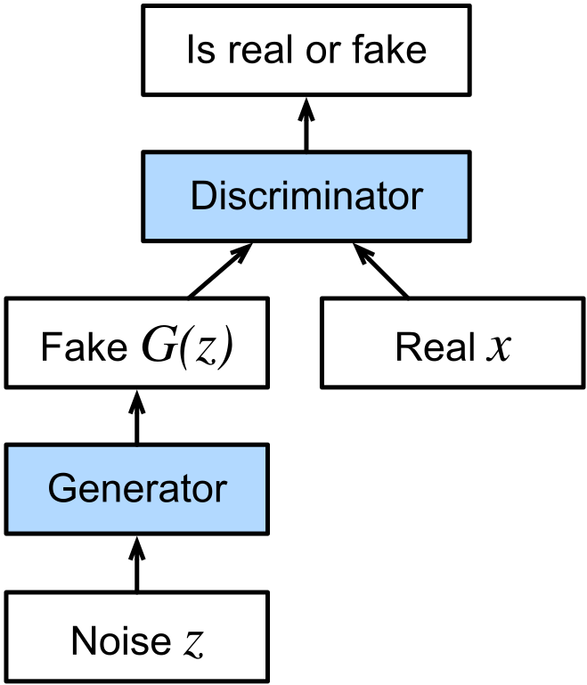
GANs rely on a dual-network setup, where two neural networks are trained simultaneously in a competitive process, often described as a two-player adversarial game:
-
Generator (
): The generator takes random noise as input and transforms it into a data sample that resembles those in the training set. Its objective is to “fool” the discriminator by producing outputs indistinguishable from real data. -
Discriminator (
): The discriminator evaluates whether a given sample is real (from the training data) or fake (produced by the generator). It is trained to distinguish between genuine samples and those generated by .
These two networks are in direct competition. The generator aims to maximize the likelihood of the discriminator being “fooled,” while the discriminator strives to minimize its error in distinguishing real samples from fake ones. This adversarial interplay ensures that the generator improves its ability to create realistic outputs over time.
Loss Function in GANs
The key innovation of GANs lies in how the loss function is defined. Since evaluating the realism of an image is inherently subjective and complex, the discriminator itself is used to define the loss for the generator.
The discriminator is trained using a binary classification loss:
- It maximizes the probability of correctly identifying real samples as real.
- Simultaneously, it minimizes the probability of classifying generated samples as real.
The generator, in turn, is trained to minimize the discriminator’s ability to distinguish between real and generated data. Formally, the training process can be described as a minimax optimization problem:
where,
Training Generative Adversarial Networks (GANs)
GAN training involves iteratively improving two neural networks: the generator (
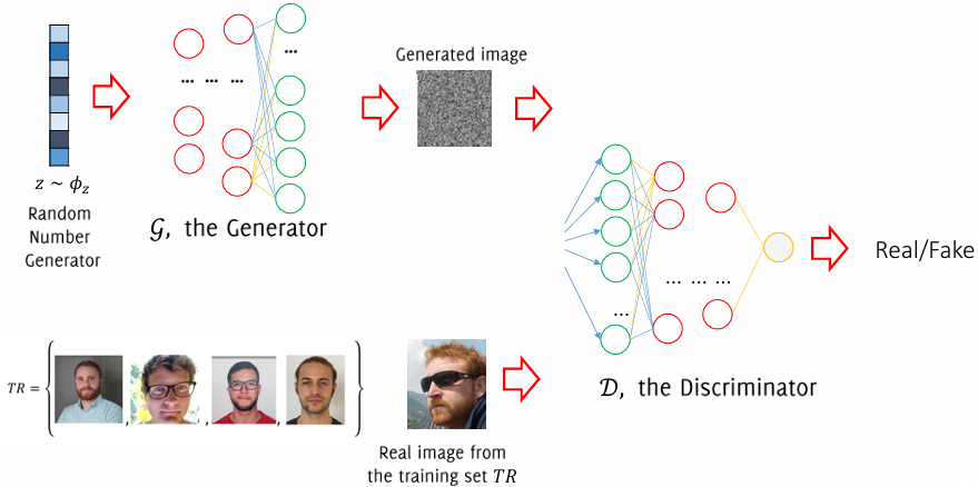
Both
The outputs of the networks are as follows:
, providing the likelihood of a sample being real. , generating images from the latent noise space.
An effective discriminator satisfies:
is maximized for real samples . is maximized for fake samples generated by . is maximized when .
Training involves solving a minimax optimization problem:
The discriminator is trained to maximize the binary cross-entropy loss, ensuring that real samples are assigned high probabilities and generated samples low probabilities. The generator, in turn, is trained to minimize the loss, effectively making it harder for the discriminator to identify generated samples as fake. This can be solved by an iterative numerical approach, where we alternate:
-steps of stochastic gradient ascent with respect to , keep fixed and solve: -step of stochastic gradient descent with respect to being fixed: and since the first term does not depend on , this consists in minimizing:
Algorithm
Minibatch stochastic gradient descent training of generative adversarial nets. The number of steps to apply to the discriminator,
, is a hyperparameter. We used , the least expensive option, in our experiments.
for number of training iterations do
for
steps do
- Sample minibatch of
noise samples from noise prior . - Sample minibatch of
examples from data generating distribution . - Update the discriminator by ascending its stochastic gradient:
end for
Sample minibatch of
noise samples from noise prior . Update the generator by descending its stochastic gradient:
end for
The gradient-based updates can use any standard gradient-based learning rule. We used momentum in our experiments.
Optimization Steps:
-
Discriminator Update:
For-steps, fix and optimize using stochastic gradient ascent: -
Generator Update:
Fixand perform one step of stochastic gradient descent on : To address vanishing gradients when
is close to zero early in training, an alternative objective can be used: which provides stronger gradients for
during early training stages.
Challenges and Remarks
- Instability: Training GANs is inherently unstable, requiring careful synchronization of generator and discriminator updates. Techniques like Wasserstein GAN (WGAN) improve stability by modifying the loss function.
- Gradient Updates: Training relies on standard optimization tools such as backpropagation and dropout.
- Evaluation: Quantitatively assessing the generator’s performance is challenging since the model provides implicit representations. Likelihood metrics cannot be directly computed.
- Implicit Generative Model: The generator does not explicitly model the data distribution but learns to map noise to realistic samples.
- Final Model: After training,
is discarded. The generator, combined with the noise distribution , serves as the generative model.
GAN Inference
Once training is complete, the primary objective is for the generator (
At the conclusion of training, the discriminator is discarded, as its purpose was solely to guide the generator during the adversarial process. The generator is retained as the final model capable of producing realistic samples. This shift reflects the core goal of GANs: to develop a standalone generator that can synthesize data indistinguishable from the original dataset.
Key Outcomes of GAN Inference
-
Discriminator Role:
The discriminator is no longer necessary after training. It was designed to distinguish real samples from fake ones during the adversarial learning process. However, its utility ends with training, as its parameters and performance are not required to produce new data. -
Performance of the Generator:
By the end of training,should generate realistic samples that closely mimic the training set’s data distribution. Importantly, the generator achieves this without having seen any specific training sample directly. It only learns to map random noise ( ) to the data space based on feedback from . -
Training Implications:
The success ofimplies that the discriminator, which was effective during training, becomes less capable of distinguishing between real and generated samples. This indicates that the generator has reached a level of proficiency where its outputs are indistinguishable from the real data as judged by the discriminator. -
Standalone Generative Model:
The generator functions independently post-training. It combines the learned transformationand the predefined noise distribution to produce new samples. This approach makes it possible to synthesize novel data without explicit reference to the original dataset.
Once trained, GANs serve as powerful tools for generative tasks. The generator can be used for various applications, including data augmentation, image synthesis, and solving inverse problems like inpainting or super-resolution.
Conditional Generative Adversarial Networks (Conditional GANs)
Conditional GANs (cGANs) extend the standard GAN framework by incorporating auxiliary information, such as class labels or other metadata, to guide the generative process. In this setup, every image in the training set
To leverage this auxiliary information, it is integrated into both the generator and discriminator architectures. The goal is to steer the image generation process in a controlled manner, ensuring that the output aligns with the given label
Incorporating Auxiliary Information
In the generator (
In the discriminator (
By introducing this conditional structure, the discriminator learns to classify as “fake” any generated image whose content does not align with the encoded class label. On the other hand, it identifies real images as consistent with their labels, thus reinforcing the importance of label-content alignment.
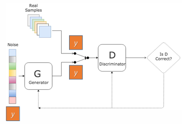
The conditional structure ensures that generated images are consistent with their labels in two ways:
-
Generator Training:
The generator is penalized during training whenever the discriminator classifies its outputs as inconsistent with the given label. This feedback encouragesto produce images that align with the auxiliary information. -
Discriminator Structure:
By appending label information to the input images, the discriminator is explicitly trained to evaluate the alignment between an image’s content and its label. It learns to distinguish not just real from fake images but also correct from incorrect label-content pairs.
Applications and Advantages
Conditional GANs are particularly valuable in scenarios requiring controlled image generation. For instance, in datasets with multiple classes, cGANs enable class-specific image synthesis, such as generating a specific type of animal or a particular digit. This capability is essential for applications like:
- Data Augmentation: Creating balanced datasets by synthesizing images for underrepresented classes.
- Style Transfer and Customization: Generating content tailored to specific user preferences or attributes.
- Interactive Generative Models: Allowing users to specify desired attributes or features during the generation process.
GANs for Anomaly Detection
Generative Adversarial Networks have proven to be effective in learning a mapping between random variables and the manifold of natural images. This ability of GANs to model complex data distributions can be harnessed for tasks beyond image generation, such as anomaly detection.
In the context of anomaly detection, we aim to identify deviations from normal patterns within images, which can be crucial for applications like industrial defect detection, medical imaging, and surveillance. GANs can be trained to generate only normal (non-anomalous) images, and by using this model, we can then detect anomalies in new, unseen images.
The GAN Framework for Anomaly Detection
Suppose we are given a training set
The challenge in anomaly detection is identifying regions in a given image that deviate from the expected normal patterns. To do this, we would ideally like to be able to invert the mapping of the generator, i.e., to find the latent vector
Let’s define
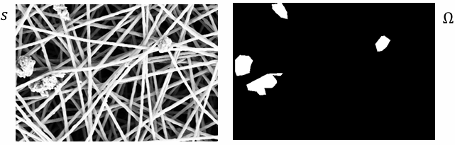
The key idea is that if we could invert the GAN’s generator
However, directly inverting
Once we have a method for obtaining a latent representation of the image through
Formally, the anomaly score for an image
where,
Bidirectional GANs (BiGANs)
Bidirectional GANs (BiGANs) extend the traditional GAN framework by introducing an encoder
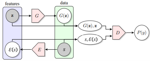
The objective function of a BiGAN is designed to encourage both the generator and encoder to work together to achieve an optimal mapping. The discriminator
Formally, the BiGAN optimization problem is defined as follows:
where the objective function
where,
Anomaly Detection with BiGANs
One of the potential applications of BiGANs is in anomaly detection. The encoder
Thus, an image
Alternatively, the discriminator’s output can be used as an anomaly score. Since the discriminator is trained to distinguish between real and fake pairs of images and latent vectors, it will likely classify anomalous images as fake. Therefore, the posterior probability
While the basic approaches described above are effective, there are more sophisticated ways to compute anomaly scores using BiGANs. One such method combines both reconstruction loss and latent space distance, leading to a more robust anomaly score.
The reconstruction loss measures how well the image
In addition to the reconstruction loss, we can also compute a term that measures the distance between the latent representations of the discriminator. Specifically, we measure the difference between the latent representations of the original image and the generated image in the latent space. This distance is calculated as:
where
where,
Limitations of BiGANs
Despite their effectiveness, BiGANs have several limitations that need to be addressed:
-
Image-wise / Patch-wise Training: BiGANs typically operate on image-level data and may struggle to identify anomalies at smaller scales, such as specific patches within an image. To address this, BiGANs could be adapted to perform patch-wise anomaly detection, but this requires additional changes to the architecture and training process.
-
Training Stability: Like traditional GANs, BiGANs can suffer from instability during training. Careful tuning of hyperparameters and the use of techniques like Wasserstein loss or gradient penalty can help improve stability.
-
Reconstruction Quality: While BiGANs can generate reconstructions of input images, the quality of the reconstructed images may not always be ideal. Unlike autoencoders, which are specifically trained for reconstruction, BiGANs may not optimize for reconstruction quality, which can be a limitation when high-quality reconstructions are required.
Fully Convolutional Anomaly Detection by GANs
In the context of anomaly detection, fully convolutional GANs (FC-GANs) can be an efficient and powerful solution. By using convolutional layers throughout the model, these networks are able to process images in a way that is computationally efficient, while maintaining a high level of performance for detecting anomalies.
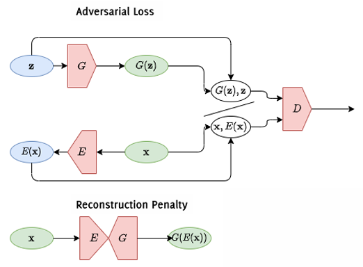
Training
In FC-GANs, all the layers of the generator and discriminator are fully convolutional, which means they use convolutional operations instead of fully connected layers. This design choice makes the model more efficient, particularly for image data, since convolutional layers are designed to capture local patterns and spatial hierarchies effectively. Additionally, convolutional networks can handle images of varying sizes, which further enhances the model’s flexibility.
To ensure stability during training, least squares (LS) losses are often used. This is a modification of the traditional GAN loss, where the discriminator’s objective is to minimize the least squares error instead of the binary cross-entropy loss. This approach has been found to improve the stability of GAN training, reducing issues like mode collapse, where the generator produces limited or low-quality outputs.
Inference
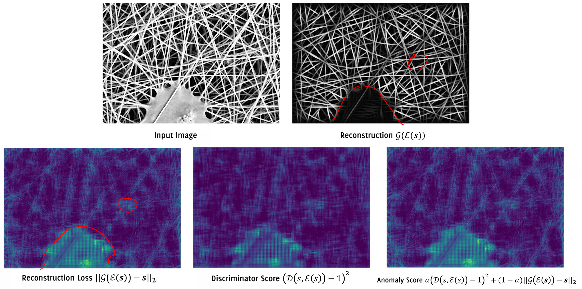
During inference, anomaly detection relies on several key factors. The anomaly score is typically computed using two main components:
- Image Reconstruction Error:
The generator is tasked with reconstructing the input image
after it has been encoded into a latent space by the encoder . The reconstruction error measures the difference between the original image and its reconstruction. This error is computed as the -norm:
A high reconstruction error suggests that the image
- Discriminator Loss:
The discriminator
is designed to distinguish between real and fake image-latent vector pairs. For normal images, the discriminator should ideally output a value close to 1, indicating that it believes the pair is real. Anomalous images, however, will produce a lower score. The discriminator loss, which measures the difference between the discriminator’s output and the ideal value of 1 for real images, is computed as:
This loss term encourages the model to identify images that deviate from the normal distribution, contributing to the anomaly score.
- Likelihood with Respect to the Estimated Distribution:
Optionally, the likelihood of the latent representation
under the distribution of latent vectors can be considered. If the latent vector for a given image has a low likelihood under , it suggests that the image is anomalous. This likelihood can be combined with the reconstruction and discriminator losses to refine the anomaly score.
The final anomaly score can be expressed as:
Advantages of Fully Convolutional GANs for Anomaly Detection
-
Efficiency: Fully convolutional networks are much more efficient for processing images, as they make use of shared weights and local receptive fields, reducing the computational burden compared to fully connected networks.
-
Flexibility: Since convolutional layers can handle varying image sizes, FC-GANs are more flexible and can be used for anomaly detection across different types of image datasets.
-
Improved Stability: The use of least squares losses helps improve training stability, which is often a challenge in standard GANs.
-
Detailed Anomaly Detection: By leveraging both image reconstruction error and discriminator loss, FC-GANs are able to more accurately detect anomalies in images, even those that are subtle or have small, localized anomalies.
DALL-E2 and SORA: Advanced Generative Models
DALL-E2: Text-to-Image Generation
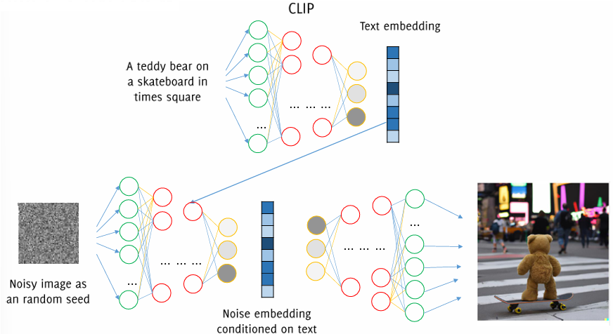
DALL-E2, developed by OpenAI, represents a significant advancement in generative models, specifically designed to create highly realistic images from textual descriptions. Building on the foundation laid by its predecessor, DALL-E, this model leverages the power of transformer architectures and large-scale training datasets to generate images that are not only visually coherent but also contextually accurate based on the input text. DALL-E2’s ability to interpret detailed and complex textual prompts allows it to generate a broad range of images, from everyday objects to abstract concepts.
A distinguishing feature of DALL-E2 is its text-to-image generation capability, which allows users to provide textual descriptions that the model then translates into images. This functionality has vast potential for creative and practical applications, as it enables users to visualize ideas and concepts without needing artistic expertise. For example, a simple text prompt like “a cat wearing a space suit” would result in the generation of a corresponding image. The model is able to produce a variety of images that are not just visually plausible but also match the conceptual intent expressed in the input text.
Moreover, DALL-E2 excels in generating high-resolution images with fine details, enhancing the realism of the content. The generated images can range from photorealistic depictions to artistic interpretations, making the model versatile across various domains. The model’s ability to produce diverse outputs from a single prompt also allows for exploration in creative industries, where multiple iterations or versions of a concept are often needed.
SORA: Self-Organizing Recursive Algorithm
SORA, or Self-Organizing Recursive Algorithm, is a novel approach to generative modeling that introduces self-organization and recursive learning principles into the generative process. Unlike traditional GANs, which rely on a static generator and discriminator framework, SORA employs a recursive framework that iteratively refines its outputs. This iterative process improves the quality and coherence of the generated samples over successive generations, making it particularly effective in scenarios where the data distribution is complex, multi-modal, or difficult to model with conventional techniques.
At the core of SORA is its recursive learning approach, where the model undergoes multiple stages of refinement. In each iteration, the model generates an initial sample and then uses feedback from the previous generation to improve the output. This recursive nature ensures that the final result is more coherent and accurate than what would be achievable with a single pass through the model. The ability to refine the outputs over time makes SORA suitable for tasks that require high-quality, detailed, and consistent outputs, such as image synthesis, texture generation, and other forms of data augmentation.
Additionally, SORA emphasizes self-organization, meaning the model can autonomously discover and represent the underlying structure of the data without explicit supervision. This capability allows it to adapt to the data’s inherent complexity and multi-modality, which is often challenging for traditional models. Self-organization is particularly beneficial when the dataset exhibits diverse patterns that require the model to dynamically adjust its approach to capturing different aspects of the data.
Due to its flexibility and adaptability, SORA is a versatile tool for a wide range of generative tasks, from image synthesis to data augmentation and anomaly detection. Its recursive and self-organizing nature positions it as a powerful alternative to traditional GANs and other generative models, especially when dealing with complex data distributions.
Comparing DALL-E2 and SORA
While both DALL-E2 and SORA represent cutting-edge advancements in generative modeling, they approach the task of generating data from different perspectives. DALL-E2 is primarily focused on text-to-image generation, translating textual descriptions into realistic images. It excels in its ability to create diverse and detailed images based on textual input, making it highly useful for applications that require visualizing concepts from language. In contrast, SORA leverages recursive learning and self-organization, refining its outputs iteratively and adapting to complex data structures. Its flexibility allows it to be applied to a wider variety of generative tasks, such as image synthesis, texture generation, and data augmentation.