4.1 - Convolutional Neural Network (CNN)

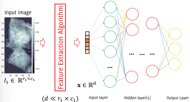
In the realm of image classification, raw images cannot be directly input into classifiers. This limitation necessitates an intermediate step known as feature extraction, which serves to distill meaningful information from the original data while simultaneously reducing its dimensionality. The essence of feature extraction lies in identifying and selecting the most relevant characteristics of an image that can contribute to effective classification. The quality of these extracted features is paramount; the more representative and informative they are, the more accurately a classifier can perform.

Feature extraction can involve various methodologies, including hand-crafted features. These are manually designed attributes that capture specific aspects of the images. For instance, one might consider attributes such as average height, area (defined by the coverage of non-zero measurements), distribution of heights, perimeter, and diagonals. In the context of a neural network, an image must be transformed into a vector , where is significantly smaller than . This transformation is executed through a feature extraction algorithm, often represented as the initial layer in a Convolutional Neural Network (CNN). Upon completion of the training process, the output layer of the network will provide the probabilities indicating the likelihood that the image belongs to a particular class.

It is crucial to distinguish between the processes of feature extraction and classification. Feature extraction is typically a hand-crafted endeavor, relying on prior knowledge and expert insights to determine the features deemed important for classification. In contrast, the classification process is fundamentally data-driven; the neural network learns to recognize patterns and make predictions based on the training data it encounters. When examining hand-crafted features, it is essential to recognize both their advantages and disadvantages.

Hand-crafted Features Pros	Hand-crafted Features Cons
Leverage expert knowledge	Extensive design and programming effort required
Features are interpretable	Not suitable for many visual recognition tasks
Allows for performance adjustments	Risk of overfitting the training set
Emphasize specific relevant features	Lack of portability across different datasets

Convolutional Neural Networks

Local Linear Filters

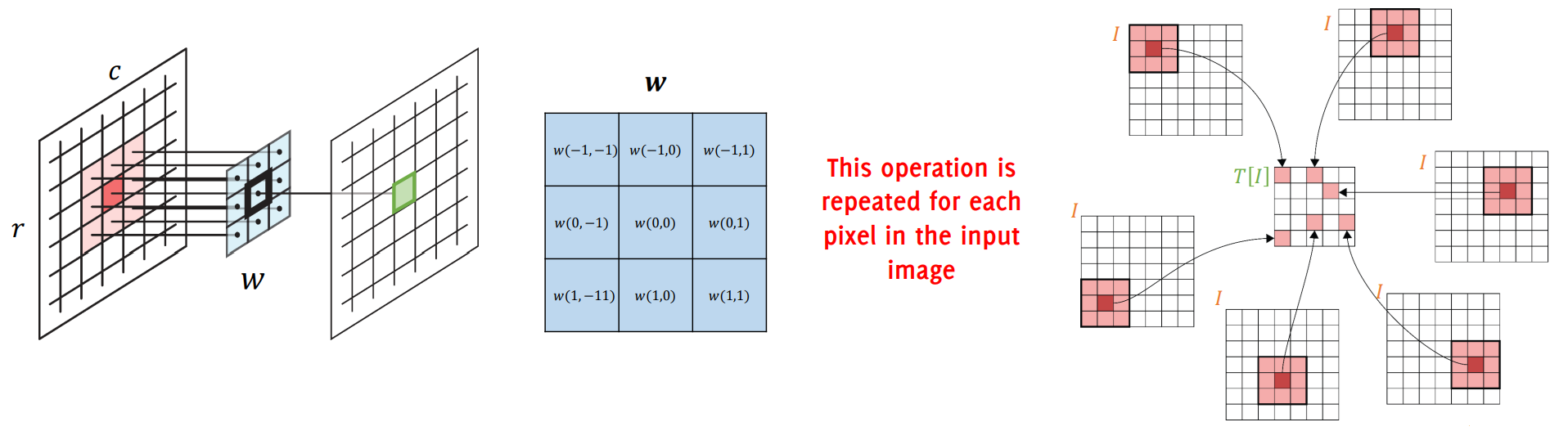
In the context of CNNs, local linear filters play a crucial role in transforming input images into feature maps. A linear transformation operates under the principle of linearity, which implies that the output at each pixel is computed as a linear combination of the pixel values in a neighborhood :

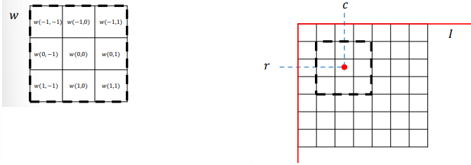
where, represents a set of weights, often visualized as an image or a filter . The filter is integral to defining the linear transformation , as it dictates how pixel values in the input image contribute to the transformed output.

2D Correlation

Convolution is a fundamental operation in CNNs that extends the concept of linear transformation to two dimensions. It is mathematically expressed as follows:

In this equation, is the input image, is the filter, and the convolution operation applies the filter uniformly across all pixels. This uniform application means that the same filter is used at each pixel position, effectively capturing local patterns in the image.

It's important to note that convolution can be viewed as a 2D correlation operation with an additional "flip" of the filter .

However, in the context of CNNs, this flipping is typically not implemented explicitly.

The process of convolution is intrinsically linked to the Fourier theorem, which emphasizes the necessity of considering filter flipping when calculating convolution in the frequency domain. Yet, in practical CNN arithmetic, this flip is often omitted, simplifying the implementation.

Padding

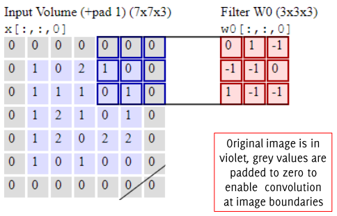
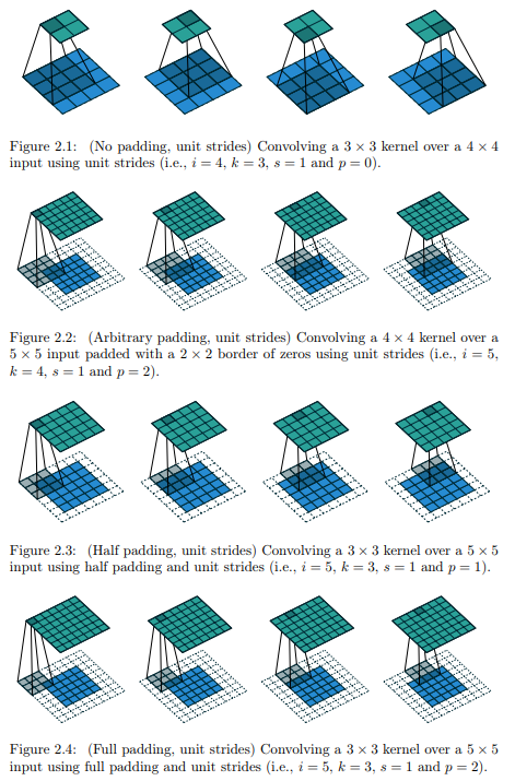
One of the key challenges in convolution is how to define the output near the boundaries of the input image. To address this, padding techniques are employed. Zero-padding is the most commonly used method, where the image is surrounded by a border of zeros. This approach preserves the spatial dimensions of the output feature map. Other options include no padding or symmetric padding, where the input image is mirrored at the edges, allowing the filter to operate effectively even near the boundaries.

Stride

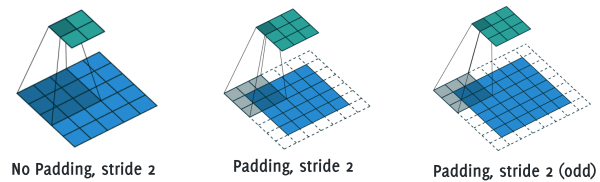
While the concept of stride is not frequently applied in traditional filtering, it plays a significant role in CNN architectures. Stride refers to the step size by which the filter moves across the input image during convolution. A larger stride results in a more significant reduction of the spatial dimensions of the output feature map. In essence, applying a stride can be viewed as a combination of convolution followed by down sampling, leading to a more compact representation of the input data. This technique not only helps to control the size of the output but also aids in reducing the computational load, allowing for deeper and more complex neural networks.

Typical CNN Architecture

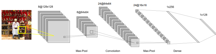
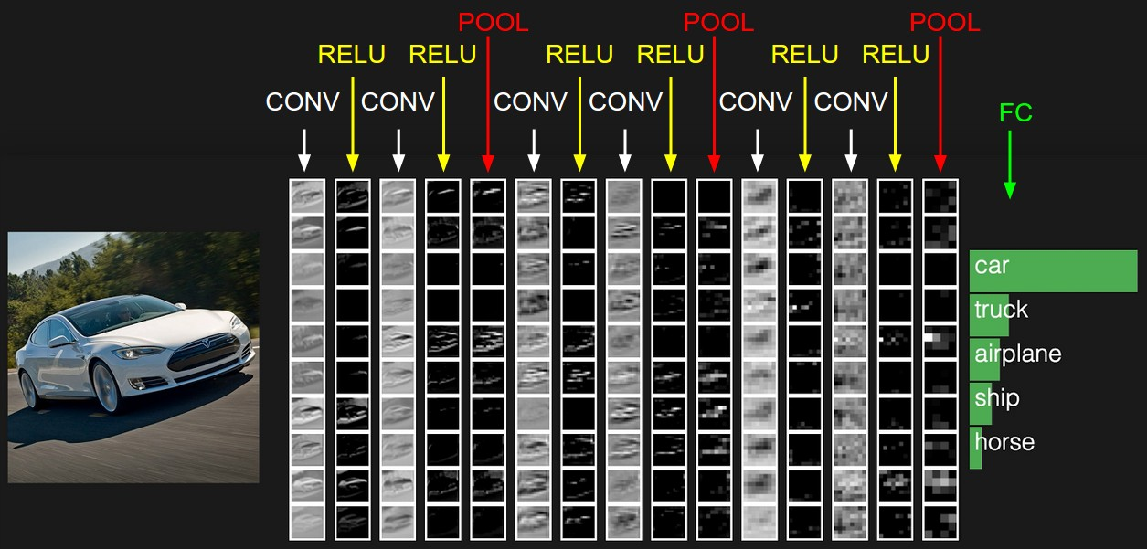
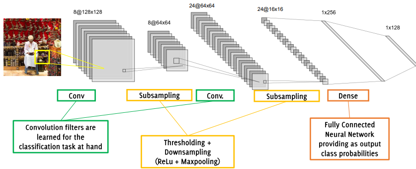
CNNs are structured as a series of interconnected blocks, each serving a specific purpose in the transformation of input images into higher-level feature representations. The fundamental components of a typical CNN architecture include convolutional layers, activation functions (nonlinearities), and pooling layers (such as subsampling or max pooling). This layered approach enables the network to learn and extract increasingly complex features from the input data.

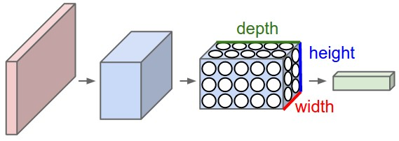
As an image traverses through the layers of a CNN, it undergoes a series of transformations, ultimately resulting in a sequence of volumetric representations. The architecture is designed such that, as the depth of the network increases, the spatial dimensions (height and width) of these volumes decrease while the depth (or the number of channels) increases. This transformation can be broken down into several key steps:

1. Input Layer: The process begins with the input of a complete image, which serves as the initial data for the CNN. This image typically consists of pixel values representing its color and intensity.

2. Convolutional Layers: In the first stage, the image is convolved with multiple filters. Each filter is designed to detect specific features, such as edges, textures, or shapes. The result of this convolution operation is a set of feature maps, each highlighting different aspects of the original image. This process allows the network to capture essential patterns at various spatial resolutions.

3. Increase in Channels and Decrease in Spatial Size: As the image passes through successive layers of the network, the number of feature maps (or channels) generated increases. Simultaneously, the spatial dimensions of these maps decrease due to the effects of convolution and pooling operations. The pooling layers, in particular, are responsible for downsampling the feature maps, reducing their height and width while retaining the most salient features. This dimensionality reduction helps the network focus on the essential characteristics of the image while also improving computational efficiency.

4. Flattening: Once the image has been transformed into a series of feature maps, it is eventually flattened into a vector. This vector serves as a compact representation of the learned features, ready to be passed on to traditional neural networks (NNs) for further processing. At this stage, the network may employ fully connected layers, which help in making predictions based on the extracted features.

Convolutional Layer

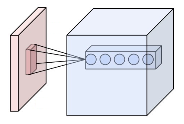
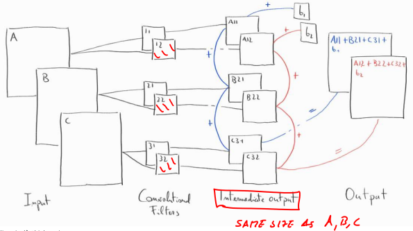
In convolutional neural networks, the convolutional layer plays a pivotal role in processing input data by mixing all components of the input. Specifically, the output of a convolutional layer is computed as a linear combination of pixel values from a localized region of the input image, spanning all its channels. This means that each convolutional filter applies its weights over a small spatial area but processes the entire depth of the input.

The operation performed by a convolutional layer can be described mathematically as follows:

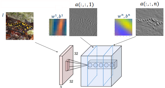
In this equation, represents the activation at location in the first output channel, represents the weights (the filter) applied over the spatial neighborhood and across the depth , and is the bias term. This filter is applied uniformly across the entire input image, resulting in a new feature map or “slice” of the output volume.

To ensure that the convolution operates across all channels of the input, the filter must have the same depth as the input volume. For instance, if the input image has 3 channels (e.g., RGB), each convolutional filter must also span 3 channels. The spatial dimensions of the filter, denoted as , cover a small localized region such as a or grid. These spatial dimensions are an essential hyperparameter in the design of convolutional layers.

Each filter yields a separate feature map in the output. For instance, the second output feature map is given by:

Thus, different filters applied at the same layer produce different channels in the output volume. The filters in a convolutional layer have the same spatial extent but are individually responsible for different aspects of the input data.

Definition

The generalized form of the convolutional operation in a CNN can be written as:

Where:

• denotes the activation at position in the output feature map ,
• is the filter for the -th output channel,
• refers to the input values in the spatial neighborhood across all channels .

In this context:

• represents the spatial dimensions of the filter, typically a small area like or ,
• is the number of channels in the input, corresponding to the depth of the input volume.

The number of parameters in a convolutional layer is calculated as:

Where is the size of the filter, is the number of input channels, and is the number of filters. Each filter has associated weights and a bias term, contributing to the total parameter count.

Python Example: Defining a Convolutional Layer

In a typical CNN implementation, convolutional layers are defined using deep learning libraries such as TensorFlow. An example of a convolutional layer in Python using TensorFlow Keras might look like this:

conv2 = tfkl.Conv2D(filters = n_f, 
					kernel_size = (h_r,h_c), 
					activation = 'relu', 
					strides = (1,1), 
					padding = 'same', 
					name = 'conv2')

where:

• n_f refers to the number of filters in the layer,
• kernel_size defines the spatial dimensions of the filters,
• strides controls the movement of the filter across the input, and
• padding = 'same' ensures the output has the same spatial dimensions as the input.

CNN Arithmetic

To illustrate the parameter calculations:

• Consider a convolutional layer with a single input map and a filter size of . This configuration produces one output map.
• If the number of filters is increased to 2, the output will consist of 2 feature maps.
• If the number of input maps (channels) is increased to 3, and there are still 2 filters, the total number of filters would be (since each filter spans all channels of the input), leading to parameters, plus 2 biases for each filter, for a total of 152 parameters.

Activation Layers

Activation layers introduce nonlinearity into neural networks, which is crucial for enabling the model to learn and represent complex patterns in data. Without these nonlinearities, the network would effectively behave like a linear classifier, limiting its capacity to model intricate relationships in the data. Activation functions are applied to each element in the output volume individually, and they do not alter the dimensions of the volume.

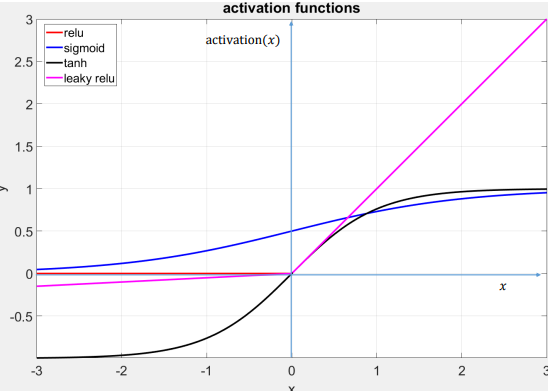
The ReLU function is by far the most widely used activation function in deep neural networks, particularly after its success in the AlexNet architecture. It is a simple thresholding function that outputs the input directly if it is positive, and outputs zero otherwise:

ReLU is popular because it introduces nonlinearity while being computationally efficient. It also mitigates the vanishing gradient problem found in older activation functions like sigmoid and tanh, making it easier for networks to propagate gradients during backpropagation.

However, ReLU can suffer from the dying neuron problem, where neurons become inactive (outputting zero) and stop responding to any input, particularly during training when a large number of neurons output zero and fail to recover. This issue can occur if the neuron consistently receives negative input, effectively “killing” it.

Leaky ReLU is a variant of the ReLU function designed to address the dying neuron problem. Instead of zeroing out negative values, it assigns them a small, non-zero slope, typically a small positive value such as . This allows some information to pass through even when the input is negative:

Leaky ReLU helps avoid neurons becoming completely inactive and is often used as an alternative to ReLU in situations where the dying neuron problem is observed.

The Tanh activation function squashes input values into a range between and . Unlike ReLU, which zeroes out negative inputs, Tanh provides a smooth transition between negative and positive values, making it differentiable:

Tanh is useful in tasks where the output needs to be centered around zero, but it suffers from the vanishing gradient problem, particularly in deeper networks. As inputs grow large in magnitude (either positive or negative), the gradient of the function approaches zero, slowing down the learning process.

The Sigmoid function is another nonlinear activation function, which squashes inputs into the range . It is differentiable and continuous, making it a popular choice in earlier neural network architectures and for binary classification tasks:

Similar to Tanh, Sigmoid suffers from the vanishing gradient problem because the slope of the function diminishes as the input grows large, making it harder for the network to update the weights during training.

In convolutional neural networks, ReLU and its variants like Leaky ReLU are the most commonly used activation functions due to their ability to efficiently introduce nonlinearity without significantly slowing down training. Tanh and Sigmoid are less popular in CNNs but are often used in multilayer perceptron (MLP) architectures or in specific parts of a network (e.g., output layers for binary classification tasks).

Pooling Layers

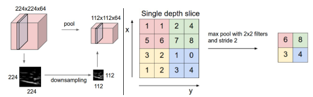
Pooling layers are essential in convolutional neural networks (CNNs) for reducing the spatial dimensions of the input volume, helping to make the network computationally efficient while retaining the most important features. Pooling operates independently on each depth slice of the input (i.e., each channel) and reduces the size of the spatial dimensions by summarizing regions, typically through a max pooling operation. This reduces the number of parameters and controls overfitting, all while maintaining critical information.

In a typical max pooling operation with a filter, the layer examines non-overlapping blocks of four values (in 2D) and retains the maximum value from each block, effectively discarding 75% of the input values. This is done for each depth slice separately. The resulting volume has smaller spatial dimensions but retains the same number of depth channels.

Pooling layers typically use strides equal to the pooling filter size. For example, a max pooling layer with a filter and a stride of reduces both the width and height of the input by half. This reduction in spatial size (by 25%) allows the network to become deeper and more computationally efficient as the spatial size decreases with each pooling layer.

It is also possible to specify a different stride for the pooling operation. For instance, using a stride of 1 means the filter slides over the input one pixel at a time without reducing the spatial size. This is known as overlapping pooling and can be useful when finer granularity in feature extraction is needed, although it is computationally more expensive.

Pooling can be done with other operations such as average pooling, where the average of each block is computed instead of the maximum, but max pooling is more common because it retains the most prominent features. Pooling layers, particularly nonlinear pooling like max pooling, are crucial for downsampling while preserving important patterns.

Dense Layers

Dense layers, also called fully connected (FC) layers, are employed towards the end of a CNN architecture after several convolutional and pooling layers have transformed the input into a high-level representation. In this layer, the spatial dimensions are flattened into a 1D vector, and every neuron (output unit) is connected to every neuron in the previous layer, just as in a traditional multilayer perceptron.

This full connection is why the layer is called “dense” — it connects all input neurons to all output neurons. The dense layer typically outputs a vector whose size equals the number of target classes, making it ideal for classification tasks. Each value in this output vector represents the network’s “confidence score” for the input belonging to a particular class.

Dense layers are particularly powerful because they combine and process all features learned by the convolutional layers to make final predictions. However, they also come with a large number of parameters, making them computationally expensive. For this reason, dense layers are often the most parameter-heavy part of a CNN, even though they are only used after the spatial dimensions have been sufficiently reduced by convolutional and pooling layers.

LeNet: The First Convolutional Neural Network

LeNet, developed by Yann LeCun in 1998, was the pioneering architecture of Convolutional Neural Networks, primarily designed for recognizing handwritten digits in the MNIST dataset. This architecture was groundbreaking because it demonstrated how CNNs could automatically learn features from raw pixel data, eliminating the need for manually designed feature extraction. The simplicity and elegance of LeNet have made it an essential reference for understanding modern deep learning architectures.

One of the key insights behind LeNet was avoiding the use of each individual pixel as a separate input to a large Multilayer Perceptron. Since images are highly spatially correlated (i.e., neighboring pixels share meaningful patterns), treating each pixel as an independent feature would ignore the inherent structure. CNNs, on the other hand, preserve the spatial structure of the input through convolutional operations, making them highly effective for visual tasks.

Architecture of LeNet

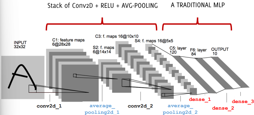
LeNet’s architecture consists of two convolutional layers followed by three fully connected layers. It gradually reduces the spatial dimensions of the input while increasing the depth, leading to compact feature representations that are suitable for classification.

1. C1 (Convolutional Layer):

   • 6 filters, each of size , applied to the input with a stride of 1.
   • Uses a ReLU activation function to introduce nonlinearity.
   • The result is a set of 6 feature maps of size , since no padding is applied and the input size is reduced from .

2. S2 (Average Pooling Layer): An average pooling operation is applied with a filter size of and a stride of 2, reducing the spatial size to while maintaining the 6 feature maps.

3. C2 (Convolutional Layer):

   • 16 filters, each of size , applied to the pooled feature maps from S2, producing 16 feature maps of size .
   • Again, ReLU is applied to introduce nonlinearity.

4. S4 (Average Pooling Layer): Similar to S2, an average pooling layer is applied with a filter, reducing the size to .

5. Flattening: The output from the convolutional and pooling layers is flattened into a vector of 400 values, which serves as the input to the fully connected layers.

6. Dense Layers: Three fully connected layers follow:

   • The first dense layer has 120 units, applying the ReLU activation function.
   • The second dense layer has 84 units, also using ReLU.
   • The final dense layer has 10 units (corresponding to the 10 digit classes in MNIST), with a activation to provide class probabilities.

Here’s a Python implementation of the LeNet architecture using Keras:

from keras.models import Sequential
from keras.layers import Dense, Flatten, Conv2D, AveragePooling2D
 
num_classes = 10
input_shape = (32, 32, 1)
 
model = Sequential()
model.add(Conv2D(filters=6, kernel_size=(5, 5), activation='tanh', input_shape=input_shape, padding='valid'))
model.add(AveragePooling2D(pool_size=(2, 2)))
model.add(Conv2D(filters=16, kernel_size=(5, 5), activation='tanh', padding='valid'))
model.add(AveragePooling2D(pool_size=(2, 2)))
model.add(Flatten())
model.add(Dense(120, activation='relu'))
model.add(Dense(84, activation='relu'))
model.add(Dense(num_classes, activation='softmax'))

Layer-wise Parameter Calculation

Layer (type)                  Output Shape        Param # 
=================================================================
conv2d_1 (Conv2D)             (None, 28, 28, 6)   156
_________________________________________________________________
average_pooling2d_1 (Average  (None, 14, 14, 6)   0 
_________________________________________________________________
conv2d_2 (Conv2D)             (None, 10, 10, 16)  2416
_________________________________________________________________
average_pooling2d_2 (Average  (None, 5, 5, 16)    0 
_________________________________________________________________
flatten_1 (Flatten)           (None, 400)         0 
_________________________________________________________________
dense_1 (Dense)               (None, 120)         48120 
_________________________________________________________________
dense_2 (Dense)               (None, 84)          10164 
_________________________________________________________________
dense_3 (Dense)               (None, 10)          850 
=================================================================
Total params: 61,706
Trainable params: 61,706
Non-trainable params: 0

• C1 Layer (Convolution): The number of parameters for the first convolutional layer is (5x5 filters for each of the 6 feature maps, plus biases).

• C2 Layer (Convolution): The number of parameters for the second convolutional layer is .

• Fully Connected Layers:

  • Flattened input from the previous layers results in 400 units.
  • First dense layer: parameters.
  • Second dense layer: parameters.
  • Output layer: parameters.

Total Parameters:

Impact of Padding and Filters

In LeNet, no padding is applied in the first convolutional layer. This reduces the size of the feature maps as they pass through the layers, from to and further down. The absence of padding is not problematic in this case, as the outer pixels of the input are black (in the MNIST dataset), and hence contain minimal information.

CNN vs MLP for Image Classification

If we were to use a traditional MLP instead of a CNN, treating each pixel as an independent input feature, the number of parameters would explode:

• For a grayscale image (1024 pixels), feeding directly into an MLP with 84 hidden units would result in parameters.
• If the input were an RGB image, the number of input pixels would increase to , tripling the number of parameters.

In contrast, CNNs limit the number of parameters by leveraging the spatial locality of image pixels. In CNNs, the filter size governs the parameter count, and only the number of parameters in the first convolutional layer increases when moving from grayscale to RGB. For instance, the filter size in the first layer increases from to , and hence, the number of parameters changes accordingly:

Thus, CNNs significantly reduce the parameter count compared to MLPs, especially as the input dimensionality grows.

---

References

• A guide to convolution arithmetic for deep learning
• Convolutional Neural Networks (CNNs / ConvNets)
• Visualizing what ConvNets learn
• 2018 Turing Award