6 - Convolutional Neural Networks for Object Detection

Object Detection: Principles and Techniques

Object detection is a fundamental task in computer vision that involves identifying and localizing objects within an image. For an image , the goal is to assign it multiple labels drawn from a fixed set of categories , with each label corresponding to an instance of an object present in the scene. Additionally, the task requires identifying the coordinates of a bounding box that encloses each object instance. Formally, object detection aims to map the input image to a set of outputs, each describing an object instance as a tuple of bounding box parameters and a class label:

This process must account for an unknown and varying number of objects in the image. The task entails drawing bounding boxes around each object and assigning them appropriate class labels based on a predefined set of categories.

Multi-Label Classification in Object Detection

In contrast to single-label classification tasks, where an image is assigned one label from a set of mutually exclusive categories, object detection often involves multi-label classification. An image can simultaneously contain instances of multiple object categories. Most conventional convolutional neural networks are designed to produce a fixed-sized output for a single-label classification task. However, they can be adapted for multi-label classification by modifying the architecture and training approach.

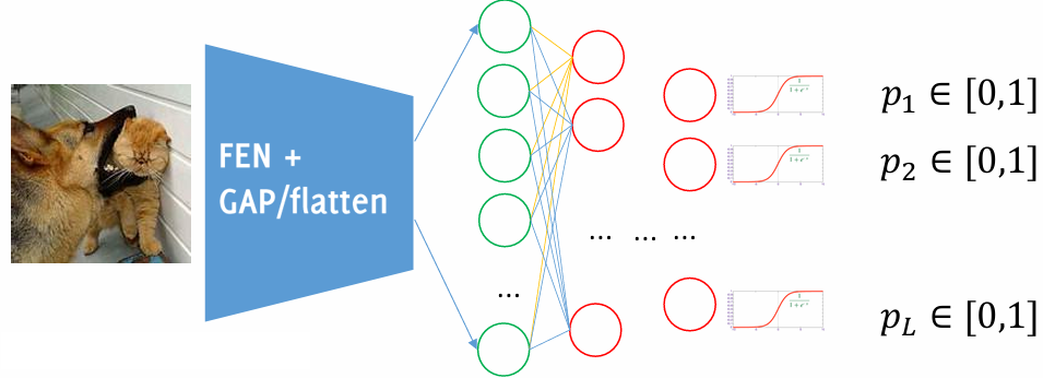
To enable multi-label classification, the softmax activation function in the output layer is replaced with a sigmoid activation function in each of the output neurons. The ^th neuron then predicts a probability , representing the likelihood of the input image containing the ^th category.

Unlike softmax, these probabilities do not sum to one, allowing for non-exclusive predictions where the image might belong to multiple categories simultaneously.

Training such a model requires using the binary cross-entropy loss function. This loss evaluates each output neuron independently, ensuring that the model learns the probabilities for multiple labels in a consistent manner.

The Sliding Window Method

The sliding window technique is a foundational method for object detection and has parallels to approaches used in semantic segmentation. This method involves using a pretrained CNN designed for fixed-sized inputs, such as , to classify regions of an image. The image is systematically divided into overlapping windows or crops, each of the same fixed size, and the pretrained model is applied to classify the content of these regions.

An important aspect of this approach is the inclusion of a “background” class in the set of categories, ensuring that regions without objects are appropriately classified. By leveraging existing CNNs without additional training, this method provides a direct application of standard classification networks to object detection.

While conceptually simple, the sliding window approach has several drawbacks:

1. Inefficiency in Feature Reuse
   Overlapping crops result in redundant computations, as the features shared between neighboring regions are repeatedly processed. This leads to significant inefficiencies, especially when dealing with high-resolution images.

2. Challenges in Choosing Window Size
   A single fixed window size may not adequately capture the diverse scales of objects within an image. Small objects might be overlooked, while large objects might not fit within the crop, reducing detection accuracy.

3. Scale Variations
   Addressing objects of different sizes requires processing a vast number of crops with varying window dimensions, which exponentially increases the computational load.

Despite its inefficiency, the sliding window approach offers one notable advantage: it does not require retraining the CNN. Pretrained models can be directly applied, making it an accessible and straightforward method for proof-of-concept implementations or scenarios with limited training resources.

Region Proposal

Region proposal methods offer a more targeted approach to object detection, addressing many limitations of the sliding window technique. These algorithms aim to identify specific regions in an image that are likely to contain objects, significantly reducing the number of regions that need to be classified.

Before the advent of deep learning, traditional region proposal algorithms, such as Selective Search, were used to generate bounding boxes with high recall but relatively low precision. These algorithms relied on heuristics and handcrafted features to identify candidate object regions.

Modern deep learning-based approaches, such as Region Proposal Networks (RPNs), have replaced traditional algorithms. These networks integrate region proposal generation directly into the CNN pipeline, enabling end-to-end training and improved accuracy. The process involves two key steps:

1. Generating Region Proposals
   A region proposal algorithm identifies candidate bounding boxes in the image. These proposals serve as potential locations for objects.

2. Classification of Proposal Regions
   The content within each proposed region is classified using a CNN. This step determines the object category and refines the bounding box coordinates.

R-CNN: Object Detection Through Region Proposals

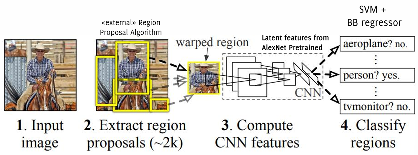
R-CNN, short for “Regions with Convolutional Neural Networks,” represents a pioneering approach to object detection that combines region proposal techniques with deep learning. It tackles the object detection problem by identifying regions of interest (ROIs) in an image and applying CNN-based classification and bounding box refinement to these regions.

1. Region Proposals
   R-CNN relies on external algorithms, such as Selective Search, to generate region proposals. These algorithms identify candidate bounding boxes that might contain objects. While they achieve high recall (ensuring most objects are captured), they lack learning capability, making them suboptimal for precision.

2. Warping to a Predefined Size
   Since R-CNN uses fully connected layers in its bounding box regression CNN, input regions must be resized to a fixed dimension. This warping step standardizes the input size but may distort smaller objects or cause loss of spatial detail.

3. Pretrained CNN for Feature Extraction
   A pretrained CNN, such as AlexNet or VGG16, is used to extract features from each region proposal. The network is fine-tuned to detect a specific set of object classes (e.g., 21 PASCAL VOC classes instead of the 1,000 ImageNet categories).

4. Classification with SVM
   After feature extraction, a linear Support Vector Machine (SVM) is trained to classify the extracted region features. Unlike modern approaches, R-CNN uses post-hoc training for SVM, which is not integrated into the end-to-end learning pipeline.

5. Bounding Box Regression
   A regression network refines the bounding box coordinates proposed by the ROI algorithm. This step ensures more precise localization of objects.

6. Background Class
   To filter out regions that do not correspond to objects, R-CNN includes a background class in the classifier.

Loss Function and Performance Metrics

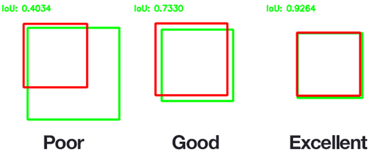
R-CNN evaluates its performance using the Intersection over Union () metric, which measures the overlap between predicted and ground truth bounding boxes. IoU is computed as:

The model’s loss function, , quantifies the discrepancy between the predictions () and the ground truth annotations (). This loss accounts for several factors:

• Missed Detections: Instances where objects are not detected.
• False Positives: Incorrectly identifying regions as objects.
• Bounding Box Accuracy: The closeness of predicted bounding boxes to ground truth, measured via IoU.

Despite its contributions to object detection, R-CNN has several drawbacks that limit its efficiency and scalability:

1. Training Inefficiencies

   • R-CNN employs separate training stages for fine-tuning the CNN, training SVMs, and bounding box regression. These ad-hoc objectives prevent end-to-end optimization, resulting in a cumbersome workflow.
   • Training is time-intensive, taking approximately 84 hours, and requires significant disk space to store intermediate features.

2. Inference Bottlenecks

   • During inference, the CNN must process each region proposal individually. This leads to redundant computations, as features are not shared across overlapping regions.
   • As a result, inference is slow, with detection times reaching 47 seconds per image when using VGG16.

3. Dependence on External Region Proposals
   The region proposal step relies on algorithms like Selective Search, which are not optimized for the object detection pipeline. This disjointed integration limits the model’s overall efficiency and accuracy.

4. Limited Scalability The need to process a large number of proposals (often thousands per image) makes R-CNN unsuitable for real-time applications or scenarios requiring high throughput.

Fast R-CNN

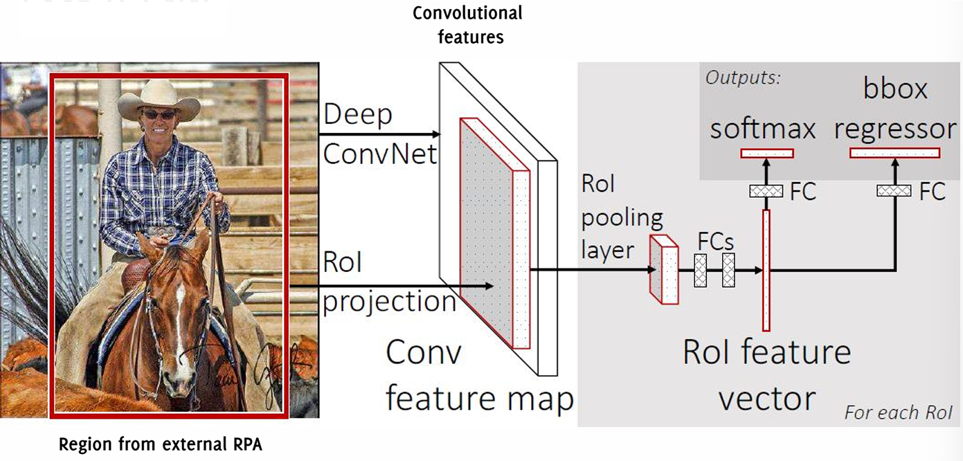
Fast R-CNN improves upon the inefficiencies of the original R-CNN by introducing a streamlined architecture that significantly reduces computational redundancy and enables end-to-end training. This model achieves faster training and inference while maintaining accuracy, making it a pivotal step in the evolution of object detection.

1. Single Pass Through the Image
   Instead of processing individual region proposals independently, the entire image is passed through a CNN to extract feature maps. These feature maps capture spatial and semantic information about the image in a compact representation, ensuring that overlapping regions reuse shared computations.

2. Region Proposals Mapped to Feature Maps
   Region proposals are projected directly onto the extracted feature maps rather than the original image. This mapping enables the model to leverage the computational efficiency of shared features.

3. Region of Interest (ROI) Pooling
   To handle the variable sizes of region proposals, Fast R-CNN introduces ROI pooling layers. Each projected region in the feature maps is divided into a fixed grid. A max-pooling operation is applied within each grid cell to generate a fixed-size output for every ROI. This ensures compatibility with fully connected (FC) layers while preserving critical spatial information.

4. Unified Classification and Bounding Box Regression
   Fast R-CNN integrates classification and bounding box regression into a single network. The FC layers process the pooled ROIs to simultaneously estimate the class probabilities and refine the bounding box coordinates. A multitask loss function combines these objectives:

   where balances the contributions of the two tasks. Unlike R-CNN, no separate SVM is required for classification, as the network directly predicts class scores.

5. End-to-End Training
   The entire network, from the convolutional layers to the ROI pooling and FC layers, is trained in an end-to-end manner. Backpropagation is applied throughout the architecture, optimizing all components simultaneously. This integrated training framework improves both efficiency and performance.

Fast R-CNN achieves a substantial speedup over R-CNN by eliminating redundant convolutional computations. Since the CNN processes the image only once, the time spent on feature extraction is dramatically reduced. Most of the test-time computation now focuses on ROI extraction and subsequent classification and regression, making the approach much faster.

Despite its advancements, Fast R-CNN retains a reliance on external region proposal algorithms. These algorithms are not optimized for the detection pipeline and remain a bottleneck during testing. While much faster than R-CNN, the model’s inference speed is still constrained by the time taken to generate region proposals.

Comparison with R-CNN

Aspect	R-CNN	Fast R-CNN
Feature Extraction	Per region (repeated)	Shared across regions
Region Proposal Mapping	From image to CNN input	From image to feature maps
ROI Size Handling	Image warping	ROI pooling
Training Framework	Multi-stage, ad hoc objectives	End-to-end
Inference Speed	Slow (~47s/image with VGG16)	Faster (~2.3s/image with VGG16)
Dependency on Proposals	External (Selective Search)	External (Selective Search)

Faster R-CNN and the Role of the Region Proposal Network (RPN)

The Region Proposal Network (RPN) is a pivotal component in the Faster R-CNN architecture, designed to replace traditional Region of Interest (ROI) extraction methods with a trainable neural network. This advancement enhances the efficiency and accuracy of object detection by focusing computational resources on the most promising regions of an image. The RPN operates as an additional module within the Faster R-CNN pipeline, leveraging shared convolutional feature maps used for classification tasks. By doing so, it integrates seamlessly into the model’s framework, reducing redundant computations.

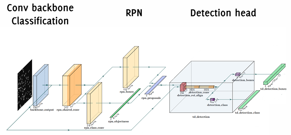
The primary goal of the RPN is to propose potential object regions, referred to as anchors, with varying scales and aspect ratios. Each spatial location in the feature map is associated with multiple anchors, typically characterized by combinations of sizes and aspect ratios. For instance, with three anchor scales and three aspect ratios, . Assuming the feature map dimensions are , the RPN produces anchor proposals, each accompanied by objectiveness scores that indicate the likelihood of containing an object.

Architecture of the RPN

The RPN architecture consists of a few key components that work together to identify and refine object proposals:

1. Intermediate Layer:
   At its core, the RPN includes an intermediate convolutional layer that takes as input the output of the feature extraction network (e.g., a pre-trained backbone like ResNet or VGG). This layer employs filters with 256 channels to process the feature maps and embed each region into a lower-dimensional space. The output feature map has dimensions , preserving spatial resolution while encoding richer semantic information.

2. Anchor Classification:
   A classification network predicts the likelihood of each anchor containing an object. For every spatial location in the feature map, the network outputs probabilities: one for the presence of an object and one for the absence. These probabilities are computed using convolutional layers followed by sigmoid activation. Each anchor’s score reflects the network’s confidence in its objectiveness.

3. Anchor Regression:
   In addition to classification, the RPN refines the anchor positions to better align with ground-truth objects. This is achieved through a regression network that predicts adjustment values for the bounding box coordinates (i.e., deltas for ). These adjustments are computed in a logarithmic space to stabilize training and facilitate convergence.

The RPN outputs proposals for each spatial location in the feature map. These proposals are characterized by:

• Objectiveness Scores: The scores for each location determine which anchors are likely to contain objects.
• Bounding Box Refinements: The adjustments refine anchor dimensions to better match the underlying objects.

To select the most promising proposals, the RPN applies non-maximum suppression (NMS). This process filters overlapping anchors based on their objectiveness scores and IoU with neighboring boxes. A fixed threshold ensures that only the top proposals are passed to subsequent stages. These proposals serve as input to the ROI pooling layer, enabling classification and bounding box regression by the Fast R-CNN head.

ROI Align and Pooling

In the Faster R-CNN architecture, ROI Align and ROI Pooling play essential roles in extracting regions from the feature maps corresponding to the proposed regions. These methods ensure that features from the Region Proposal Network are processed uniformly, regardless of the original size and shape of the proposals.

The extracted regions are subsampled or interpolated to a fixed size, allowing subsequent layers to process them in a standardized manner. For each proposal, a latent feature vector is generated, encapsulating the information within that region. This latent vector is passed to the detection head, which further processes it using fully connected layers (MLP) or convolutional layers, resulting in an ROI feature vector ready for classification and bounding box regression.

RPN and Anchor Shapes

The Region Proposal Network operates using anchors—reference bounding boxes of predefined shapes, scales, and aspect ratios. These anchors serve as the foundation for predicting objectiveness scores and bounding box adjustments.

1. Defining Anchor Targets:
   Training the RPN does not require designing separate networks for different anchor shapes or sizes. Instead, the same RPN can be trained with different target definitions that correspond to various anchor configurations. These configurations could include rectangular bounding boxes with different dimensions or even unconventional shapes.

2. Non-Rectangular Anchors:
   While the RPN can theoretically accommodate anchors of non-rectangular shapes, such as ellipses or rotated bounding boxes, practical limitations arise. Calculating the Intersection over Union (IoU) for non-rectangular shapes is computationally intensive and often lacks a closed-form solution. In contrast, rectangular bounding boxes are straightforward and efficient for computation, making them the preferred choice in most implementations.

Detection Head

The detection head is the final component of the Faster R-CNN pipeline and operates on the ROI feature vectors generated by the ROI Align/Pooling process. This module is responsible for classifying objects and refining their bounding boxes.

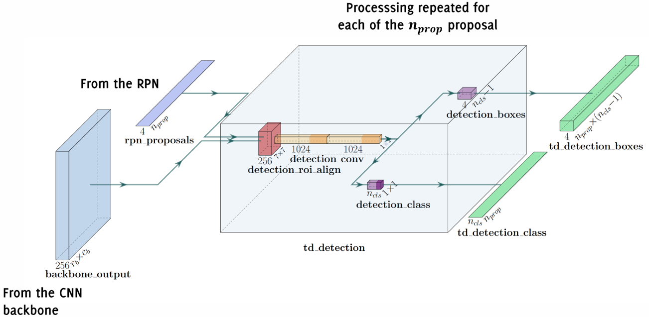
The detection head comprises two parallel branches:

1. Classification Branch:
   This branch outputs scores, where is the total number of object classes, including the “background” class. The background class serves as a placeholder for regions that do not contain any objects of interest. The classification scores represent the probability distribution over all classes for each proposal.

2. Bounding Box Regression Branch:
   The second branch predicts bounding box adjustments for object proposals. For object classes (excluding the background), this branch outputs values, representing corrections for the -coordinates, width, and height of the bounding boxes.

The detection head combines the outputs from these two branches to identify the objects with the highest confidence scores and their corresponding bounding boxes. These predictions form the final output of the Faster R-CNN model, representing the detected objects in the image.

Faster R-CNN Training Process

Training Faster R-CNN involves optimizing four main objectives, each contributing to the final performance of the model. These objectives are combined into a weighted sum to guide the training process effectively.

Loss Functions in Faster R-CNN

1. RPN Classification Loss:

   • Determines whether an anchor contains an object or not.
   • This binary classification loss is crucial for identifying promising regions.

2. RPN Regression Loss:

   • Adjusts the anchor box coordinates to better match the ground truth bounding boxes.
   • Helps improve localization accuracy.

3. Final Classification Loss: Evaluates how well the detection head classifies the proposed regions into object classes.

4. Final Bounding Box Regression Loss: Refines the bounding box coordinates output by the detection head for accurate localization.

The total loss combines these components. During training, the model uses overlap (IoU) between predicted and ground truth bounding boxes to define object/non-object targets.

Training Procedure

Faster R-CNN training proceeds in stages to handle the interdependence of the RPN and detection head effectively:

Algorithm

1. Train the RPN (Region Proposal Network):

• Freeze the backbone network and train only the RPN layers.

• Focuses on generating high-quality region proposals without considering object classes.

• Optimizes a multi-task loss combining classification (object vs. non-object) and regression (bounding box refinement).

2. Train the Fast R-CNN Detection Head:

• Use the proposals generated by the trained RPN as input.

• Fine-tune the detection head, including the backbone network, to classify and refine the proposed regions.

3. Fine-Tune the RPN:

• Refine the RPN in the context of the updated backbone network.

• Ensures the proposals are consistent with the refined feature extraction.

4. Fine-Tune the Detection Head:

• Freeze the backbone and RPN.
• Focus on training the final layers of the Faster R-CNN to improve classification and bounding box regression performance.

Inference in Faster R-CNN

At test time, Faster R-CNN operates in two stages:

1. First Stage: Region Proposal

   • Extract features using the backbone network (e.g., VGG16 or ResNet).
   • Generate approximately 300 region proposals with the RPN based on object scores.
   • Refine the bounding box coordinates of these proposals.

2. Second Stage: Detection and Refinement

   • Apply ROI pooling or ROI alignment to extract fixed-size feature maps for each proposal.

   • Use fully connected layers with a softmax to classify each ROI into object categories, including the background.

   • Predict bounding box offsets for more precise localization.

   Comparison of R-CNN, Fast R-CNN, and Faster R-CNN

   Aspect	R-CNN	Fast R-CNN	Faster R-CNN
   Feature Extraction	Per region (repeated)	Shared across regions	Shared across regions
   Region Proposal	External (Selective Search)	External (Selective Search)	Integrated (RPN)
   ROI Size Handling	Image warping	ROI pooling	ROI pooling
   Training Framework	Multi-stage, ad hoc	End-to-end	End-to-end
   Inference Speed	Slow (~47s/image with VGG16)	Faster (~2.3s/image with VGG16)	Fastest (~0.2s/image with VGG16)
   Dependency on Proposals	High	High	Low
   Efficiency	Low	Medium	High
   Accuracy	High	High	High

YOLO and SSD: Region-Free Object Detection

Object detection networks traditionally relied on region-based methods, such as R-CNN, which involve multiple sequential steps, including region proposal generation and classification. While effective, these methods are computationally expensive, require separate training for each component, and can be slow during inference. Region-free methods, such as YOLO (You Only Look Once) and SSD (Single Shot Detector), revolutionized object detection by treating it as a single-stage process, making detection faster and more efficient.

YOLO: “You Only Look Once”

YOLO reframes object detection as a single regression problem that maps raw image pixels directly to bounding box coordinates and class probabilities. Unlike region-based approaches, YOLO does not rely on separate region proposal steps. Instead, it performs detection in a single forward pass through a convolutional neural network.

Key Concepts of YOLO:

1. Grid-Based Representation
   The input image is divided into a coarse grid (e.g., ). Each grid cell is responsible for detecting objects whose center lies within it.

2. Anchors (Base Bounding Boxes)
   Each grid cell is associated with anchor boxes, or base bounding boxes, which serve as reference shapes for detecting objects. These anchors enable the network to handle objects of varying sizes and aspect ratios.

3. Predicted Outputs per Grid Cell
   For each grid cell and its associated anchors, the network predicts:

   • Bounding Box Offsets: Adjustments to the anchor box dimensions to better fit the object, represented as .
   • Objectness Score: A confidence score indicating the likelihood of an object being present in the bounding box.
   • Classification Scores: Probabilities for each object category (), including a background class.

   The network’s output has dimensions:

   where, accounts for the bounding box coordinates and objectness score, while represents the classification probabilities.

4. Single Forward Pass
   Detection is performed in a single forward pass through the network, which outputs all bounding boxes and classifications simultaneously. This design makes YOLO exceptionally fast compared to multi-step methods.

Training YOLO involves assessing a complex loss function that balances multiple objectives, such as:

• Matching predicted bounding boxes with ground truth.
• Penalizing both false positives and false negatives.
• Accounting for overlapping predictions (e.g., via Non-Maximum Suppression).

SSD: Single Shot Detector

SSD builds upon the principles of YOLO but incorporates additional mechanisms to improve detection, particularly for objects at different scales.

1. Multi-Scale Feature Maps
   SSD uses multiple feature maps at different resolutions to detect objects of varying sizes. Higher-resolution feature maps detect smaller objects, while lower-resolution maps focus on larger objects.

2. Default Boxes (Anchors)
   Similar to YOLO’s anchors, SSD defines a set of default boxes for each feature map location, varying in aspect ratio and size.

3. Predicting Offsets and Class Probabilities
   For each default box, SSD predicts:

   • Bounding box offsets.
   • Class probabilities.

4. Efficiency and Accuracy
   SSD maintains the single-shot nature of YOLO, making it faster than region-based methods. However, its use of multi-scale features generally improves accuracy compared to YOLO, particularly for small objects.

Comparison of Region-Free and Region-Based Methods

Aspect	Region-Based (e.g., R-CNN)	Region-Free (e.g., YOLO, SSD)
Pipeline	Multi-stage (region proposal + classification)	Single-stage (direct regression)
Efficiency	Slower due to multiple steps	Faster with a single forward pass
Feature Reuse	Limited (e.g., overlapping regions processed repeatedly)	High (shared feature maps)
Accuracy	Typically higher due to precise region proposals	Generally lower, especially for small objects
Training Complexity	Requires separate training for components	End-to-end, but loss function is complex

Instance Segmentation

Instance segmentation is a more advanced form of object detection, where the goal is not only to identify and classify objects within an image but also to delineate each object instance at the pixel level. This approach requires a model to handle multiple objects simultaneously, each with its own precise boundaries.

Given an input image , instance segmentation assigns:

• Multiple labels from a fixed set of categories , such as “wheel”, “car”, and so on, where each label corresponds to a distinct instance of an object.
• Bounding box coordinates for each object, indicating the location of the object within the image.
• Pixel set for each bounding box, corresponding to the object instance in the bounding box, where each pixel inside the box is assigned the appropriate label.

Definition

Formally, the image is transformed into a set of objects:

where is the number of object instances.

Instance segmentation combines the challenges of both object detection and semantic segmentation:

• Object detection: It must handle multiple instances of objects in the image, each with its own bounding box.
• Semantic segmentation: It assigns a label to every pixel in the image, including distinguishing between different object instances.

Mask R-CNN

Mask R-CNN is a powerful extension of Faster R-CNN, designed specifically for instance segmentation. While Faster R-CNN performs object detection (classifying regions and refining bounding boxes), Mask R-CNN adds an additional capability: it predicts a segmentation mask for each object instance.

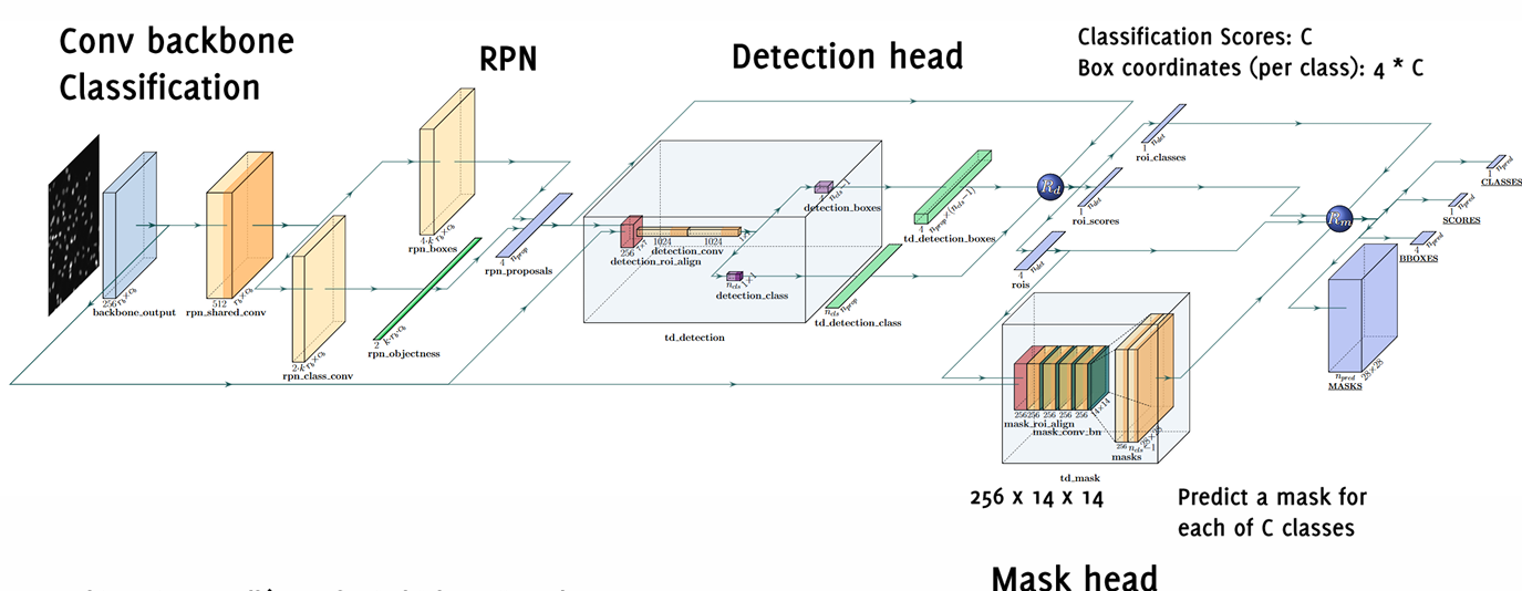
Key Components of Mask R-CNN:

1. Region Proposal Network (RPN):
   Similar to Faster R-CNN, Mask R-CNN starts by using the RPN to propose regions of interest (ROIs) in the image. These are potential object locations.

2. Bounding Box Prediction:
   As in Faster R-CNN, each ROI is classified, and the bounding boxes for each object instance are refined. The bounding box prediction is essentially an object detection task.

3. Segmentation Mask Prediction:
   The critical extension in Mask R-CNN is the addition of a parallel branch for predicting a mask for each object instance.

   • After the ROI is extracted from the feature map, it is passed through a fully convolutional network to predict a binary mask for each object.
   • This mask is of the same size as the ROI and indicates which pixels within the ROI belong to the object.

4. Parallel Processing of Bounding Boxes and Masks:
   The bounding box and mask predictions are processed simultaneously for each ROI. This means that Mask R-CNN predicts both the class and the precise object boundary in one pass, making it much more efficient than earlier segmentation methods that required separate stages for object detection and segmentation.

Training Mask R-CNN

Mask R-CNN can be trained on datasets that contain both object detection and segmentation annotations. A prominent example is the Microsoft COCO dataset, which contains over 200,000 images and annotations for 80 object categories. In addition to standard object detection annotations (bounding boxes and labels), COCO provides pixel-level segmentation masks for each object instance. The dataset also includes joint annotations for human poses, making it especially useful for training models that require fine-grained object understanding.

The training process involves optimizing multiple tasks simultaneously:

• Bounding Box Regression: Refining the position and size of the bounding boxes for each object instance.
• Classification: Determining the correct object category for each region.
• Mask Prediction: Generating a binary mask for each object instance that defines its shape at the pixel level.

The use of large, annotated datasets like COCO provides extensive training data, especially for images with many object instances. This ensures that the model can generalize well across different objects and environments.

Pros and Cons of Mask R-CNN

Pros	Cons
Precise Object Boundaries: Unlike traditional object detection methods that only predict bounding boxes, Mask R-CNN predicts pixel-level segmentation, offering detailed object outlines.	Computational Complexity: The additional mask prediction branch increases the computational load, particularly during inference. This can make Mask R-CNN slower than simpler object detection models.
Simultaneous Multi-task Learning: The architecture handles both bounding box prediction and mask prediction in parallel, making the model both fast and accurate.	Training Data Requirements: Like other deep learning models, Mask R-CNN requires large, annotated datasets for training. The process of annotating pixel-wise segmentation masks is time-consuming and resource-intensive.
Scalability: Mask R-CNN performs well on a variety of object detection tasks, from small objects to large complex scenes, due to its ability to learn both object location and shape.

Metric Learning

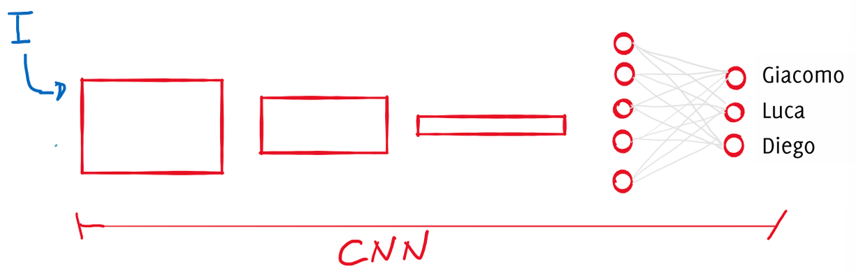
Imagine designing a face identification system to unlock a door at Bocconi University. At first glance, you might consider using traditional approaches such as classification, detection, or segmentation. However, let us take a step back and rethink the problem, beginning with a Convolutional Neural Network designed for classification. In this scenario, each individual to be recognized is treated as a distinct class. The process seems straightforward: gather a training set with a few images per class (or person), ensuring they include variations in lighting, pose, expression, and clothing. With these in hand, along with some Python code snippets and a GPU, we can train the network to classify individuals.

However, this approach quickly becomes cumbersome. Suppose a new employee joins the organization. The entire network must be retrained to accommodate the additional class, which is inefficient and impractical. A different solution arises: instead of training a model to classify images into predefined classes, why not treat the problem as one of image comparison? This can be done by storing a “template” image for each person and performing identification by comparing an input image to these stored templates.

The identification process in this template-based approach can be formulated mathematically as:

where, represents the input image, is the stored template for the ^th individual, and the system identifies the input as the person whose template is closest in terms of Euclidean distance. This approach simplifies enrollment for new individuals, as adding a new person only requires storing their template in the database.

Towards a Learned Distance

While the template-based method is intuitive and simple, it relies on raw pixel comparisons, which are often insufficient for complex tasks like face identification. A better alternative is to extract features from images using a CNN. The feature extraction process generates a latent representation , which captures meaningful patterns and abstractions about the image. These latent features are more robust for comparison than the raw image data.

In this context, identification can be performed using:

Here, and are the latent representations of the input image and the stored templates, respectively. By precomputing and storing the latent features of all templates, the system avoids redundant computations during identification. This setup effectively transforms the problem into one of image retrieval in the latent feature space, a technique known to work well in practice.

Learning a Better Distance

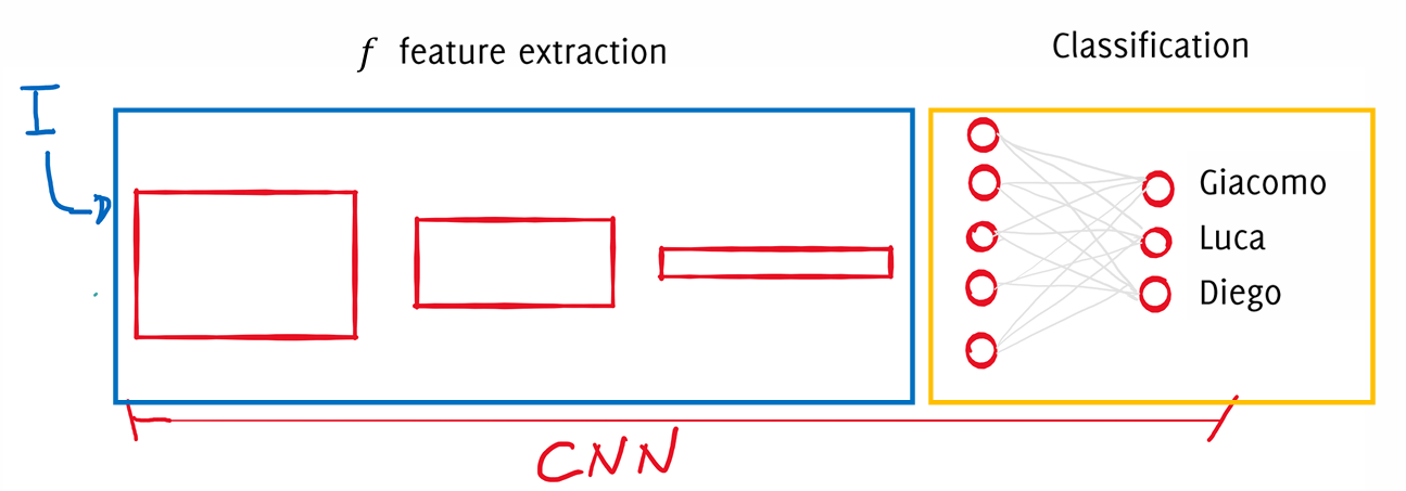
Despite its improvements, this method still has limitations. The CNN used for feature extraction was originally trained for classification, not for measuring distances between images. Consequently, the latent representations might not be optimal for comparison tasks.

To address this, we can adopt a more tailored approach by training the network explicitly to measure distances between images. The goal is to optimize the network’s parameters such that the latent space satisfies the following condition:

This means that for an input image belonging to class , its distance in the latent space to the correct template should be smaller than its distance to any other template . Achieving this requires designing a loss function and training process that encourage the network to learn a representation optimized for comparing images rather than classifying them.

The transition to a distance-based approach for face identification offers several advantages. Latent spaces trained for comparison are inherently more meaningful than those derived from classification tasks. For instance, using methods like Siamese networks or triplet loss, the network can be trained specifically to distinguish between pairs of images based on similarity. These techniques optimize the network to produce embeddings that are closer for similar images and farther apart for dissimilar ones.

In practice, this metric learning approach is widely used in modern face identification systems. It underpins technologies like FaceNet and DeepFace, enabling high accuracy in real-world scenarios with varying conditions. By leveraging a distance metric tailored to the task, these systems achieve state-of-the-art performance, transforming how face recognition and other identification systems are designed.

Siamese Networks and Contrastive Learning

Siamese networks are a specialized type of neural network architecture designed for tasks involving similarity and comparison. They consist of two identical subnetworks sharing the same weights . This weight sharing ensures that both subnetworks perform the same operations, hence the term Siamese. The primary goal is to learn a latent space where similar inputs (e.g., images of the same person) are closer, while dissimilar inputs (e.g., images of different people) are farther apart.

During training, the network is fed with pairs of images , labeled to indicate whether they belong to the same individual () or not (). The network’s parameters are optimized using a contrastive loss function, which is defined as follows:

where:

• is the label for the pair, with if the images are from the same person and otherwise.
• represents the Euclidean distance between the feature vectors of and in the latent space.
• is a hyperparameter called the margin. It defines the minimum allowable distance between dissimilar pairs in the latent space.

The loss function penalizes:

1. Similar pairs () with large distances in the latent space.
2. Dissimilar pairs () whose distance is less than the margin .

By minimizing this loss, the network learns embeddings that cluster similar images closer together while pushing apart dissimilar images, within the constraints set by .

Triplet Loss for Fine-Grained Similarity Learning

While contrastive loss is effective, triplet loss is another popular approach to learn discriminative embeddings. Triplet loss operates on triplets of images:

• Anchor (): A reference image.
• Positive (): An image of the same person as the anchor.
• Negative (): An image of a different person.

The goal is to ensure that the distance between the anchor and the positive is smaller than the distance between the anchor and the negative by a margin . The triplet loss is formulated as:

where:

• : Distance between the anchor and the positive.
• : Distance between the anchor and the negative.
• : Margin that enforces separation between similar and dissimilar pairs.

The network is trained to ensure that the positive pair is closer than the negative pair by at least , penalizing violations of this condition. This encourages robust separation in the latent space, which is critical for tasks requiring fine-grained similarity measurement, such as face identification.

Verifying a New Image

When a new image needs to be verified:

1. Feature Extraction: The image is passed through the trained network to compute its latent representation .
2. Template Matching: Identification is performed by finding the individual whose templates have the smallest average distance to the input:

3. Threshold Validation: The average distance is compared against a threshold to determine if the input matches any individual:

If the distance is smaller than , the system confirms the identity. Otherwise, it rejects the input as unidentified.

---

References

• Google Colab - Object Detection