In Convolutional Neural Networks (CNNs), the structure and role of convolutional layers are central to their power and efficiency in processing spatial data. Let’s explore the nature of parameters within a CNN, focusing first on the convolutional layers and how they differ fundamentally from the dense layers in Multi-Layer Perceptrons (MLPs). Understanding this distinction, along with concepts like sparse connectivity and weight sharing, will clarify how CNNs efficiently handle image data.
Convolutional Layers: Fundamentals and Parameter Structure
Convolutional layers in a CNN apply a “filter” or “kernel” across the input, producing an output (often called a feature map) that captures spatial relationships in the data. This process can be mathematically described as a linear combination of values within a certain region of the input, adjusted for each channel. For example, for an output feature
where
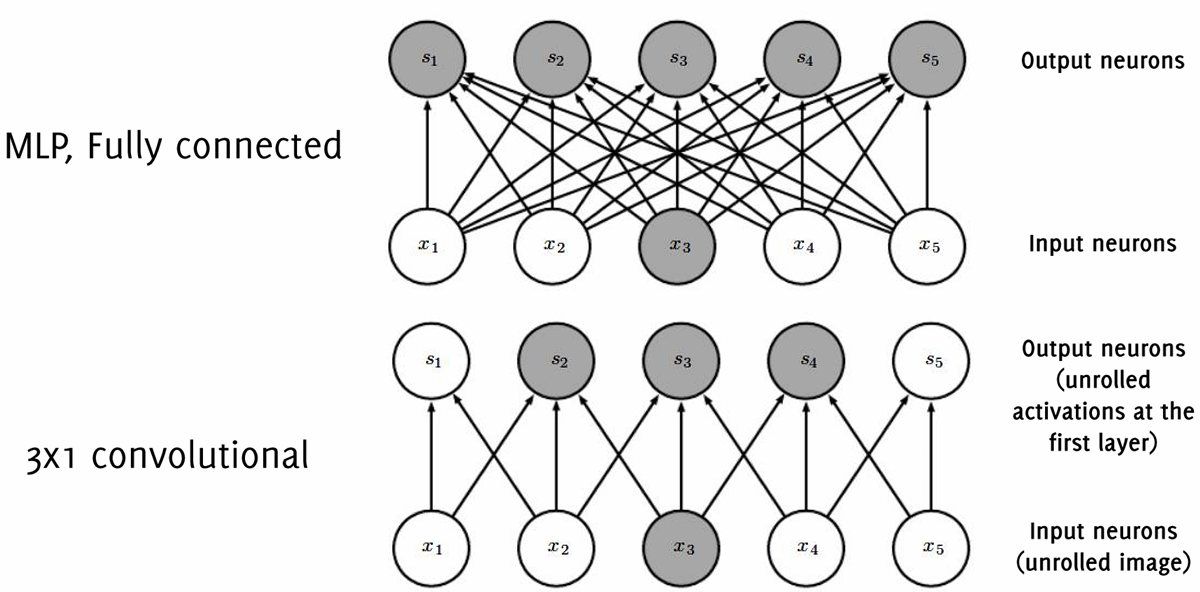
Like dense layers in MLPs, convolutional layers perform linear operations. In fact, if we were to “unroll” the input image into a vector, convolutional weights could be reinterpreted as weights in a dense layer. However, convolutional layers retain a localized structure, which limits the influence of each input value to a specific region of the output. Both layers can thus be represented in the form of a linear transformation
Differences Between Dense Layers and Convolutional Layers
Despite both layers performing linear operations, they differ notably in their parameter structures:
-
Dense Layers: Dense layers, typical of MLPs, have a fully populated weight matrix, where each input neuron is connected to every output neuron with a unique weight. Consequently, the bias term is dense as well, with a separate bias parameter associated with each output neuron. This dense connectivity allows dense layers to capture complex relationships but results in a large number of parameters.
-
Convolutional Layers: In contrast, convolutional layers are characterized by sparse connectivity. Only a subset of input neurons contributes to each output neuron, as convolutions are applied locally within a defined spatial window (typically
or ). This sparseness means most entries in the weight matrix are zero, reflecting that only nearby neurons influence each other directly. Additionally, convolutional layers use “weight sharing,” meaning the same set of weights (the filter) applies across all spatial locations. The bias term is also shared within each feature map, resulting in fewer unique parameters compared to a dense layer.
Sparse Connectivity in CNNs
The concept of sparse connectivity in CNNs means that instead of each output neuron being influenced by all input neurons, only a limited local region affects each output. This feature allows CNNs to capture spatial hierarchies in images, focusing on patterns that might occur anywhere within the input field. Because each filter detects a specific pattern or feature, only a limited set of weights is needed to learn spatial structures, which helps reduce the model complexity.
Weight Sharing and Spatial Invariance
One of the defining properties of CNNs is their spatial invariance, which stems from weight sharing. By applying the same filter weights across the entire input, CNNs are able to detect features, like edges or textures, regardless of their position in the image. This characteristic arises from the assumption that if a feature is useful to detect in one part of the image, it will likely be useful elsewhere as well. In this way, CNNs achieve spatial invariance, greatly enhancing their ability to generalize across different parts of the input.
Practical Example: Parameter Reduction in Convolutional Layers
To illustrate the efficiency of CNNs, consider an input image of
pixels with an output feature map of . If this transformation were handled by an MLP, the parameter count would be: However, in a convolutional layer, only a fraction of this number is required. For instance, a convolutional filter of size
with 6 channels would involve: This dramatic reduction in parameters is due to the use of sparse weights and shared biases, which allow CNNs to scale efficiently with the input size while retaining high expressive power for spatial features.
The Receptive Field in Deep CNNs
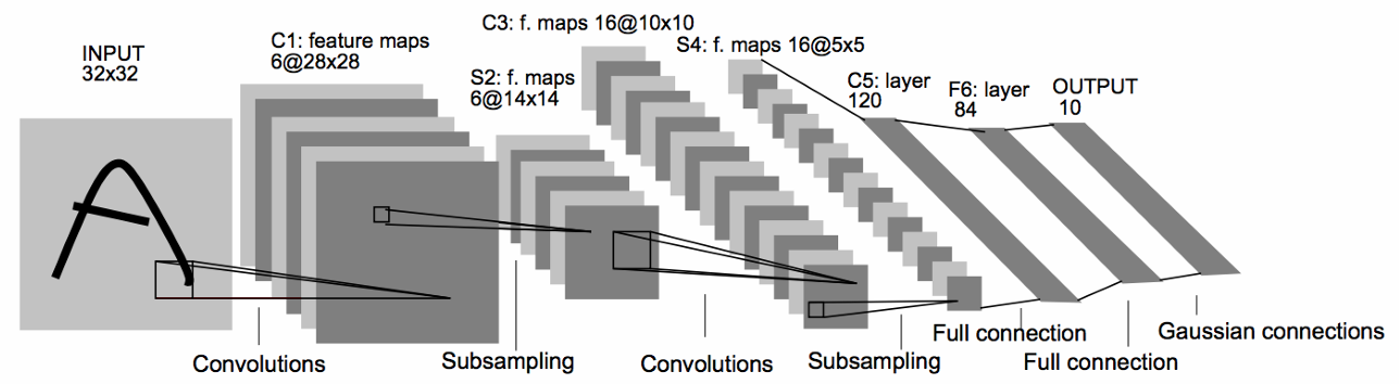
In deep Convolutional Neural Networks, the concept of the receptive field is fundamental. The receptive field refers to the specific region of the input that influences a particular output value in the network. Due to the sparse connectivity in CNNs, unlike fully connected (FC) networks where each output depends on the entire input, each output in a CNN is determined only by a localized area of the input. This localized dependence is called the receptive field, which plays a crucial role in how spatial patterns are learned and represented.
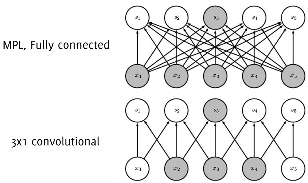
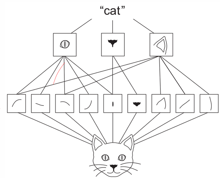
As the network depth increases, the receptive field expands. Factors like convolutional operations, max-pooling, and strides greater than one contribute to this growth, meaning that deeper layers depend on progressively larger regions of the input. Thus, neurons in these layers become sensitive to broader spatial patterns, capturing high-level features over wider areas of the image. Although the receptive field is typically considered relative to the network’s final output layer, the same concept applies to intermediate layers. As we move deeper in the network, spatial resolution decreases while the number of feature maps increases, enabling the network to detect more abstract patterns rather than focusing on precise spatial details. In short, convolution alone can enlarge the receptive field, and while max-pooling is not strictly necessary, it enhances spatial abstraction further.
Training CNNs
CNNs can be trained similarly to Multi-Layer Perceptrons (MLPs), with gradient descent to minimize a loss function such as binary cross-entropy, RMSE, or hinge loss. Although CNNs share some structural similarities with MLPs, they incorporate sparse and shared connectivities. These properties affect how gradients are computed, particularly in layers with shared weights. The backpropagation algorithm, which uses the chain rule to compute gradients, can be applied effectively in CNNs as long as each layer is differentiable.
One additional detail involves handling weight sharing in the gradient calculations, which reduces the total number of parameters to be updated. This sharing means that derivatives are computed for a limited set of weights rather than each weight being unique. For instance, during backpropagation with max-pooling, only the pixel in the receptive field that maximally contributes to the output retains the gradient, while all others are set to zero.
Example
As a specific example, consider a matrix:
Using a max-pooling operation with a
filter and stride of 2, the gradient relative to the max-pooled output would be nonzero only at the positions corresponding to the maximum values in the original input matrix, with all other positions set to zero.
The derivative for the ReLU function, a common activation function in CNNs, is similarly simplified: it is non-differentiable at zero but defined as one for positive values and zero otherwise.
A Breakthrough in Image Classification: ImageNet and AlexNet
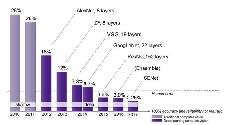
The development of deep learning has had a transformative effect on visual recognition. A major milestone in this field was the ImageNet project, a vast visual database created for advancing object recognition research. ImageNet contains over 14 million images, each manually annotated to specify the objects depicted. In addition, bounding boxes are provided for over one million images to enhance localization training. The database spans more than
The breakthrough of deep learning in visual recognition was showcased in part through AlexNet, a pioneering deep CNN that achieved unprecedented accuracy in image classification on ImageNet. AlexNet’s success was enabled by several key factors: the advent of powerful GPUs for faster computation, the emergence of frameworks like TensorFlow and PyTorch, and novel architectures that allowed the training of much deeper networks. These advances revolutionized the field of computer vision, establishing deep CNNs as the leading approach for image classification, object detection, and other visual recognition tasks.
Data Scarcity
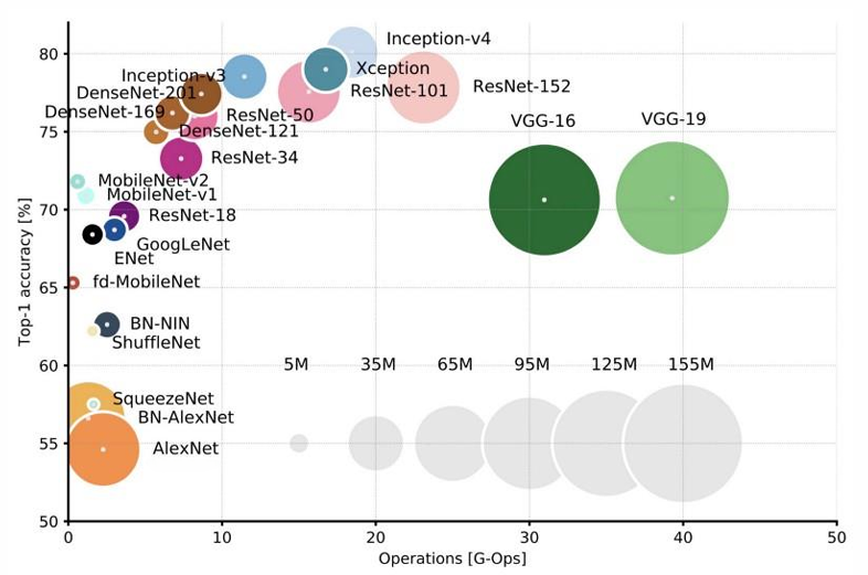
Deep learning models are highly data-intensive, requiring extensive datasets to achieve optimal performance. Networks like AlexNet, for instance, have been trained on the ImageNet dataset, which contains tens of thousands of images spanning hundreds of classes—each image in the dataset must be carefully annotated. Such a vast quantity of annotated data is essential to define the millions of parameters that characterize and enable the network to generalize across various tasks. However, when faced with a limited amount of training data, achieving similar performance can be challenging. Techniques such as data augmentation, which artificially increases the dataset by applying transformations to existing images, and transfer learning, where a model pre-trained on a larger dataset is fine-tuned for a specific task, have proven effective in addressing data scarcity.
Data Augmentation in Deep Learning
Definition
Data augmentation is a technique used to artificially expand the size and diversity of a dataset by creating modified versions of the original images.
This is especially useful in scenarios where each labeled image represents a broad class, encompassing multiple variations in appearance that should not change the label. For example, in aerial photography, images might be rotated, shifted, or scaled without altering the category. Augmentation helps improve the generalization ability of the model by teaching it to become invariant to these transformations.
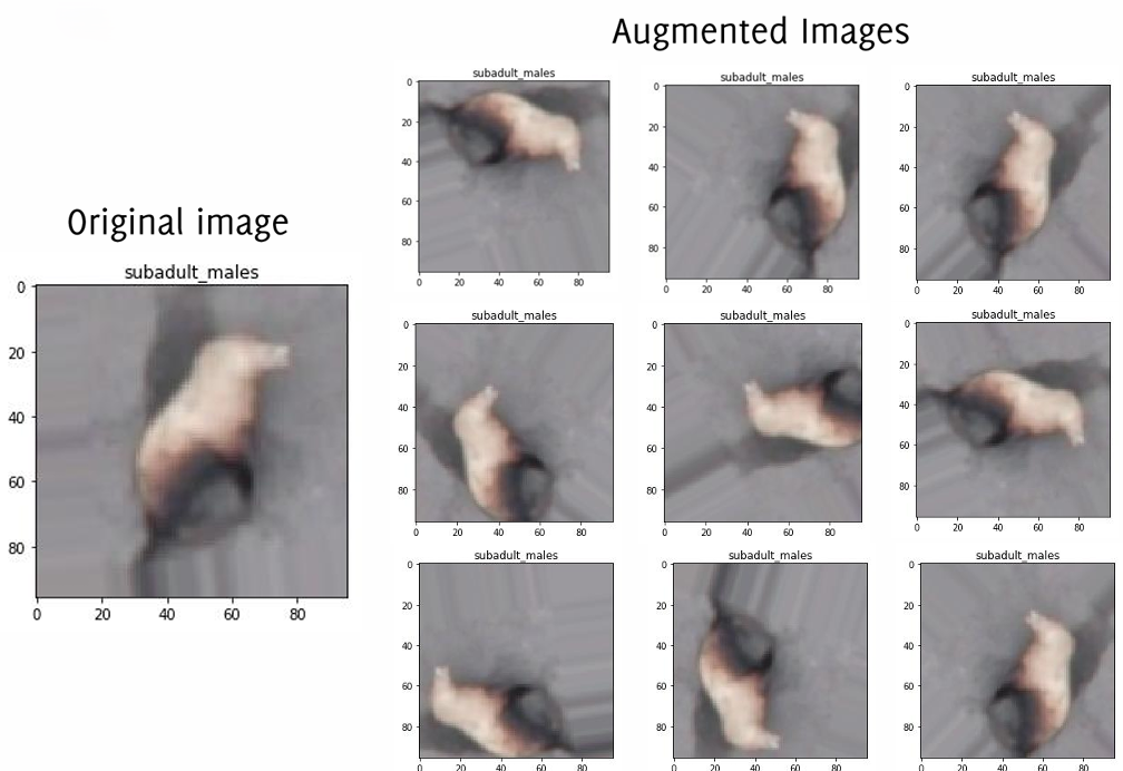
Data augmentation typically includes two types of transformations: geometric transformations and photometric transformations.
- Geometric Transformations: These involve altering the spatial properties of the images. Examples include:
- Shifts, rotations, and affine transformations: These reposition, rotate, or scale parts of the image.
- Perspective distortions and shear: These add skewing effects, changing the shape perspective.
- Scaling and flipping: These resize or mirror the image.
- Photometric Transformations: These involve modifying the pixel properties of the image. Examples include:
- Adding noise: Random noise can make the model more robust to real-world imperfections.
- Adjusting intensity and contrast: This makes the model invariant to brightness and contrast variations.
- Superimposing images: Adding elements to the image increases variability and prepares the model for potential occlusions.
For data augmentation to be beneficial, the transformations should preserve the essential characteristics of the class. If size or orientation is key for classifying or regressing on the target, applying scale or rotation must be carefully controlled. The goal is to create variations that the network will learn to ignore when they are irrelevant to classification. However, transformations that obscure distinctive features should be avoided. For instance, rotating an image of a clock without numbers would impair a model’s ability to predict the time, as the orientation provides necessary information.
Mixup Augmentation
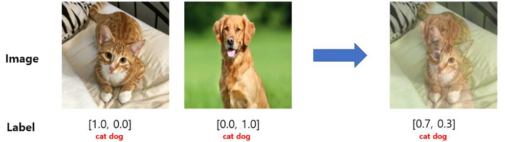
Mixup is an advanced augmentation strategy that creates virtual samples by blending two training examples.
Definition
Given two randomly selected training samples,
and , potentially from different classes, a new sample is created as follows: where
is a random value between 0 and 1, and and are one-hot encoded labels.
This technique assumes that the linear interpolations of the input features should lead to linear interpolations of their respective labels, which adds a degree of smoothness to the decision boundaries and makes the model more robust.
Implementing Mixup is simple and introduces minimal computational overhead, making it an efficient method to enhance dataset variability without the need for additional labeled data. This approach can significantly improve performance, especially when dealing with limited or imbalanced data.
Benefits of Data Augmentation
Data augmentation offers a range of benefits for enhancing model performance and robustness in deep learning, particularly when working with limited annotated data. Given an annotated image
The aim of data augmentation is to train the network to become invariant to certain transformations. Since the same label
Moreover, data augmentation alone may be insufficient to cover the full inter-class variability of images. However, incorporating augmentation into training greatly increases the dataset’s effective size, thereby reducing overfitting and enhancing the model’s generalization capability. Data augmentation can also help mitigate class imbalance by generating more realistic instances for minority classes, improving performance for classes with limited samples.
In practice, data augmentation can be implemented as a network layer that applies transformations on each batch, producing fresh augmented images in every epoch. This approach ensures that new variations are introduced continuously throughout training.
A point of caution
When data augmentation introduces patterns unique to specific classes, the model might learn these artifacts instead of actual class features. For example, if images of a particular class are consistently blurred, the network might associate “blurriness” with that class rather than focusing on its defining features. Similarly, using different color schemes, padding artifacts, or interpolation artifacts specific to certain classes may create unintended patterns that the network learns to recognize as class-specific.
Test-Time Augmentation (TTA)
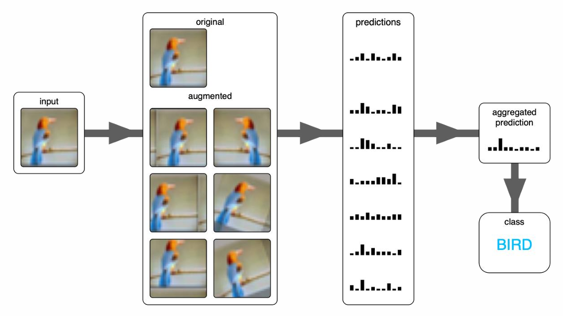
Even with augmented training data, CNNs may not achieve complete invariance with respect to the transformations. Test-Time Augmentation (TTA) is a technique used to further improve prediction accuracy by applying augmentation to test images. The steps in TTA include:
- Augmenting the test image: Generate a few random augmentations for each test image
, represented as . - Classification and posterior vectors: Classify each augmented image and record the posterior probability vectors,
. - Aggregating predictions: Compute the final prediction by averaging the posterior vectors for all augmented versions of the image, resulting in a final prediction
.
TTA can be particularly valuable for test samples where the model exhibits uncertainty, but it can be computationally demanding, as multiple inferences are performed for each test image. Therefore, it’s essential to carefully configure the types and number of transformations used at test time to optimize performance without overwhelming computational resources.
Data Augmentation in Keras
Keras offers a variety of preprocessing layers specifically designed for augmenting image data during training. These layers perform photometric and geometric transformations on images in each batch, applying random variations that help the model generalize better to real-world data. In Keras, these augmentation layers are placed right after the input layer, and they only function during training, leaving the test data untouched by augmentation.
Commonly used augmentation layers in Keras include:
RandomCrop: Crops a random portion of the image.RandomFlip: Flips the image horizontally, vertically, or both.RandomTranslation: Moves the image within a specified range.RandomRotation: Rotates the image randomly by a specified degree range.RandomZoom: Zooms into or out of the image.RandomHeightandRandomWidth: Adjust the height and width of the image.RandomContrast: Adjusts image contrast to simulate different lighting conditions.
In addition to augmentation, Keras also provides essential image preprocessing layers that are applied both during training and inference. These layers include:
- Resizing layer: Resizes images to a specified dimension, standardizing input sizes across the dataset.
- Rescaling layer: Scales pixel values, often normalizing them to a
or range, which can help improve model convergence. - CenterCrop layer: Crops the central part of the image to a specified size, useful when focusing on a specific image region.
To augment images, define a simple network that applies a single augmentation, such as a random flip:
flip = tf.keras.Sequential([
    tf.keras.layers.RandomFlip("horizontal_and_vertical"),
])
To apply this flip augmentation to a batch of training images, simply call the augmentation network:
flipped_X_train = flip(X_train)For more complex augmentations, you can stack multiple augmentation layers in sequence. Here’s an example of a network that performs a random flip, translation, and rotation:
# Combine multiple augmentation layers into a sequence
augmentationNet = tf.keras.Sequential([
    tf.keras.layers.RandomFlip("horizontal_and_vertical"),
    tf.keras.layers.RandomTranslation(0.1, 0.1),
    tf.keras.layers.RandomRotation(0.1),
], name='augmentationNet')
You can then invoke this network to augment an input batch:
augmented_X_train = augmentationNet(X_train)Keras allows augmentation layers to be incorporated directly into the model architecture. This makes augmentation an integral part of the model and applies it automatically during training. However, remember that augmentation layers will only be active during training, while preprocessing layers will also function during inference. Below is an example of a model that includes both augmentation and preprocessing:
import tensorflow as tf
from tensorflow.keras import layers as tfkl

def build_model_with_augmentation(input_shape, output_shape):
    tf.random.set_seed(seed)

    # Define input layer
    input_layer = tfkl.Input(shape=input_shape, name='Input')

    # Add augmentation layers
    a = tfkl.RandomFlip("horizontal_and_vertical")(input_layer)
    b = tfkl.RandomTranslation(0.1, 0.1)(a)
    c = tfkl.RandomRotation(0.1)(b)

    # Add a convolutional layer as an example
    conv1 = tfkl.Conv2D(filters=32, kernel_size=3, activation='relu')(c)
    # Continue defining the rest of the model...

    return tf.keras.Model(inputs=input_layer, outputs=conv1)
In this example, the augmentation layers (random flip, translation, and rotation) are applied directly to the input, followed by other layers in the model. This setup ensures that augmented versions of the data are generated in each training batch, enhancing the model’s ability to learn features that are invariant to these transformations.
Confusion Matrix
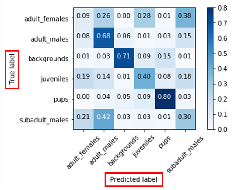
A confusion matrix is a table that illustrates the performance of a classification model by summarizing the relationship between predicted and actual classes. The element
The confusion matrix is particularly useful for analyzing the types of errors the model makes, such as whether it tends to misclassify one class as another specific class. For multi-class classification, this matrix becomes more complex, offering insight into which classes are often confused by the model.
Two-Class (Binary) Classification
In binary classification, the model’s output can be reduced to a single scalar probability, as the output probabilities for the two classes add up to one. Specifically, if the CNN produces an output vector
For binary classifiers, performance is often evaluated using the Receiver Operating Characteristic (ROC) curve, which provides a threshold-independent measure of the classifier’s ability. The ROC curve plots TPR against FPR across all possible thresholds, offering a comprehensive view of the trade-offs involved in various threshold choices. This is particularly useful when you want flexibility in setting the classification threshold, as the ROC curve shows performance independently of any specific threshold.
An ideal classifier would achieve:
- FPR = 0% (no false positives),
- TPR = 100% (all positives correctly identified).
Such a model would place the ROC curve’s optimal point at
Transfer Learning
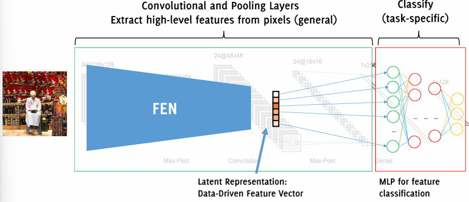
In transfer learning, the common architecture of a Convolutional Neural Network (CNN) is divided into two major sections, each playing a specific role in the model’s functionality. The first part is the feature extraction network (FEN), which is typically composed of convolutional and pooling layers designed to extract high-level features from raw pixel data. This segment generates a latent representation—a data-driven feature vector that captures the general characteristics of an image, abstracted from low-level features such as edges to complex shapes. This feature extraction is commonly trained on a large dataset, such as ImageNet, which includes a vast range of classes (often with around
The second section is a task-specific classifier, usually consisting of fully connected (FC) or dense layers, which uses the extracted features to perform the specific classification. For example, if the task is to classify images into multiple classes, the FC layer will provide a score for each class, indicating the likelihood of the image belonging to each category. This classifier’s output size is based on the number of target classes, with each neuron corresponding to a class. This approach is task-specific, which raises questions when adapting a pre-trained CNN to smaller, more specific datasets. For instance, how should the model be adjusted if the target dataset contains only cats and dogs? Or if the goal is to classify different types of sea lions? And ultimately, can the pre-trained features be applied effectively to other classification problems?
To adapt a CNN pre-trained on a large dataset to a new, more specialized task, the following steps are typically followed:
- Choosing a Pre-Trained Model: Start with a powerful pre-trained network such as ResNet, EfficientNet, or MobileNet, which has been optimized on large, general datasets.
- Removing the Fully Connected Layers: The pre-trained model’s FC layers are removed because they were designed for the initial task, with specific output classes that may not match the new task.
- Adding New Fully Connected Layers: Design and add new FC layers that match the specific requirements of the new task. These new layers are often initialized randomly, and they act as the classifier for the target problem.
- Freezing the Feature Extraction Network (FEN): By “freezing” the FEN, we prevent its weights from being modified during training on the new task, preserving the general features it has learned.
- Training Only the New Layers: With the FEN weights frozen, only the parameters of the new FC layers are trained on the target dataset.
This process, often called transfer learning, leverages the knowledge embedded in the pre-trained model to simplify training on the new task. This method is effective when limited training data is available, as it minimizes the need to update all model parameters. Common practices to maximize transfer learning include connecting a new, lightweight output layer with few parameters, training only the output layer, and enabling “fine-tuning” of the final few layers. Fine-tuning involves making the last layers trainable and adjusting them to fit the new dataset more closely. When fine-tuning the entire network, training is typically conducted at a low learning rate to refine the model without overwriting valuable pre-trained weights.
Summary
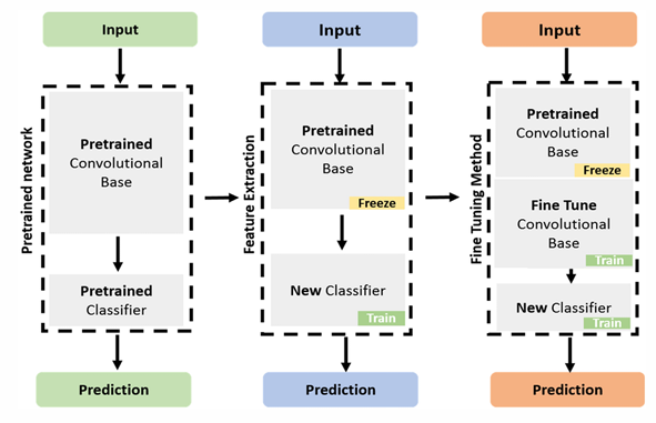
In transfer learning vs. fine-tuning, these approaches serve different purposes:
Transfer Learning: Only the newly added FC layers are trained, while the pre-trained feature extractor is frozen. This approach is optimal when the training dataset is small, and the pre-trained model is reasonably aligned with the new task.
Fine-Tuning: In this case, the entire network is retrained, with the convolutional layers initialized to the pre-trained weights. Fine-tuning is recommended when sufficient training data is available, or if the pre-trained model does not fully align with the new task. Fine-tuning typically requires a lower learning rate compared to training from scratch, as gradual adjustments are needed to avoid disrupting the previously learned features.
In Python, a typical model for fine-tuning might be compiled as follows:
# Compile the fine-tuned model
ft_model.compile(
    loss=tf.keras.losses.BinaryCrossentropy(),
    optimizer=tf.keras.optimizers.Adam(1e-5),
    metrics=['accuracy']
)
This compilation phase sets a binary cross-entropy loss, Adam optimizer, and a low learning rate to control the extent of updates on the network’s parameters, ensuring that fine-tuning can incrementally improve the model’s performance on the new task.
Transfer Learning in Keras
In Keras, transfer learning involves importing a pre-trained model and adapting it to solve a new classification task, leveraging the model’s existing feature extraction capabilities. Pre-trained models are commonly imported in two formats:
-
include_top=True: This configuration includes the entire model, with all convolutional layers and the classifier (fully connected) layers. It is intended for directly solving the original classification problem the model was trained for, such as on ImageNet. -
include_top=False: This option loads only the convolutional layers, omitting the final classifier layer. It is specifically designed for transfer learning, enabling you to attach a custom classifier layer to suit your specific task.
To load a model with Keras, you can use the following code to import VGG16 without the top layer, setting it up for transfer learning:
from keras import applications

base_model = applications.VGG16(weights="imagenet", include_top=False, input_shape=(img_width, img_width, 3), pooling="avg")
With include_top=False, the model outputs the results of a global pooling layer, which reduces the spatial dimensions. You can specify the pooling type:
pooling="avg": Global Average Pooling (GAP) to take the average of each feature map.pooling="max": Global Max Pooling (GMP) to take the maximum of each feature map.pooling="none": No pooling, returning only the raw activations.
In Keras, for sequential models, you can isolate the feature extraction network (FEN) by selecting a subset of the pre-trained model’s layers. For example, to create a FEN from the VGG16 model, excluding the last two layers:
fen = tf.keras.Sequential(base_model.layers[:-2])
print(fen.output_shape)
# Expected output: (None, 128)
Pre-trained Keras models typically expect specific input preprocessing. For example, MobileNetV2 requires
tf.keras.applications.mobilenet_v2.preprocess_input, which scales input pixel values between -1 and 1.
Transfer learning in Keras requires modifications to the model’s backend to add a new fully connected (FC) layer. Once the new layer is added, it is important to freeze the pre-trained layers so that only the newly added classifier layers are trainable.
-
Freeze Layers: Loop through the model layers and set the
trainableproperty toFalsefor all layers before a specified layer (lastFrozen).for layer in base_model.layers[:lastFrozen]: layer.trainable = False -
Example with MobileNetV2: Here’s an example of loading a pre-trained MobileNetV2 model without weights and attaching a new classifier.
# Load MobileNetV2 without the top layers mobile = tf.keras.applications.MobileNetV2(input_shape=(224, 224, 3), include_top=False, pooling='avg') -
Adding a New Top Layer: To add a new classifier layer to the model, use Keras functional API:
# Define new input layer
inputs = tf.keras.Input(shape=(224, 224, 3))
x = mobile(inputs)  # Pass input through MobileNet feature extractor
x = tf.keras.layers.Dropout(0.5)(x)  # Add dropout to prevent [[2 - Neural Networks Training and Overfitting|overfitting]]
outputs = tf.keras.layers.Dense(1, activation='sigmoid')(x)  # New output layer for binary classification

# Create the model
model = tf.keras.Model(inputs=inputs, outputs=outputs)
In this configuration, Dropout layers help mitigate overfitting, particularly useful when working with small datasets. The new classifier uses a Dense layer with a sigmoid activation, making it suitable for binary classification tasks.
Image Retrieval from the Latent Space
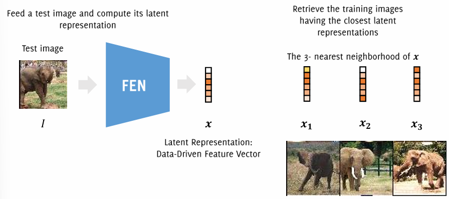
In image retrieval from the latent space, the idea is to leverage the feature extraction network’s latent representations (or embeddings) to identify images similar to a query image. By processing an input image through the FEN (in this case a pretrained AlexNet), we obtain a high-level feature vector. This vector can be used to measure similarity between the query image and other images in a training set, based on the distances between their respective feature vectors.
Steps for Image Retrieval
- Latent Representation Computation: First, pass a test image
through the FEN, obtaining its latent representation . This vector serves as a unique, data-driven feature representation of the image. - Retrieving Similar Images: To find images similar to
from the training set, compute the latent representations of all images in the training dataset. Then, identify the training images whose representations are closest to by finding the nearest neighbors (e.g., the 3 closest neighbors) based on a chosen distance metric, such as Euclidean or Manhattan distance, among all the embeddings.
1-NN Classification in Latent Space
A common approach to utilize this retrieval method is 1-Nearest Neighbor (1-NN) classification. In this method, the label of the test image
import numpy as np

# Step 1: Compute the latent representation of the test image
image_features = fen.predict(test_image)

# Step 2: Compute the latent representations of the entire training set (batch size of 512 for efficiency)
features = fen.predict(X_train_val, batch_size=512, verbose=0)

# Step 3: Calculate the distances between the test image's features and each training image's features
distances = np.mean(np.abs(features - image_features), axis=-1)  # L1 distance (Manhattan)

# Step 4: Sort the distances and get the indices of the sorted order
sorted_indices = distances.argsort()

# Step 5: Order the training images and labels based on the distance
ordered_images = X_train_val[sorted_indices]
ordered_labels = y_train_val[sorted_indices]

# Step 6: Retrieve the closest image and its label
closest_image = ordered_images[0]
closest_label = ordered_labels[0]
In this setup:
- Distance Calculation: The
np.mean(np.abs(features - image_features), axis=-1)line computes the Manhattan (L1) distance between the test image and each training image. Other distances, such as Euclidean (L2), can also be used depending on the problem requirements. - Sorted Distances: The
argsort()function sorts the distances in ascending order, providing a list of indices from the closest to the farthest images in the latent space. - Retrieving the Nearest Image: The
ordered_images[0]andordered_labels[0]lines identify the image and label of the closest match, which can then be used to classify the test image.
By ordering the training images according to their distances, you can retrieve not only the closest match but also the top K similar images, which is useful for applications beyond classification, like content-based image retrieval or similarity searches. This method is efficient and effective when your FEN is trained on a large, varied dataset, ensuring meaningful feature representations.