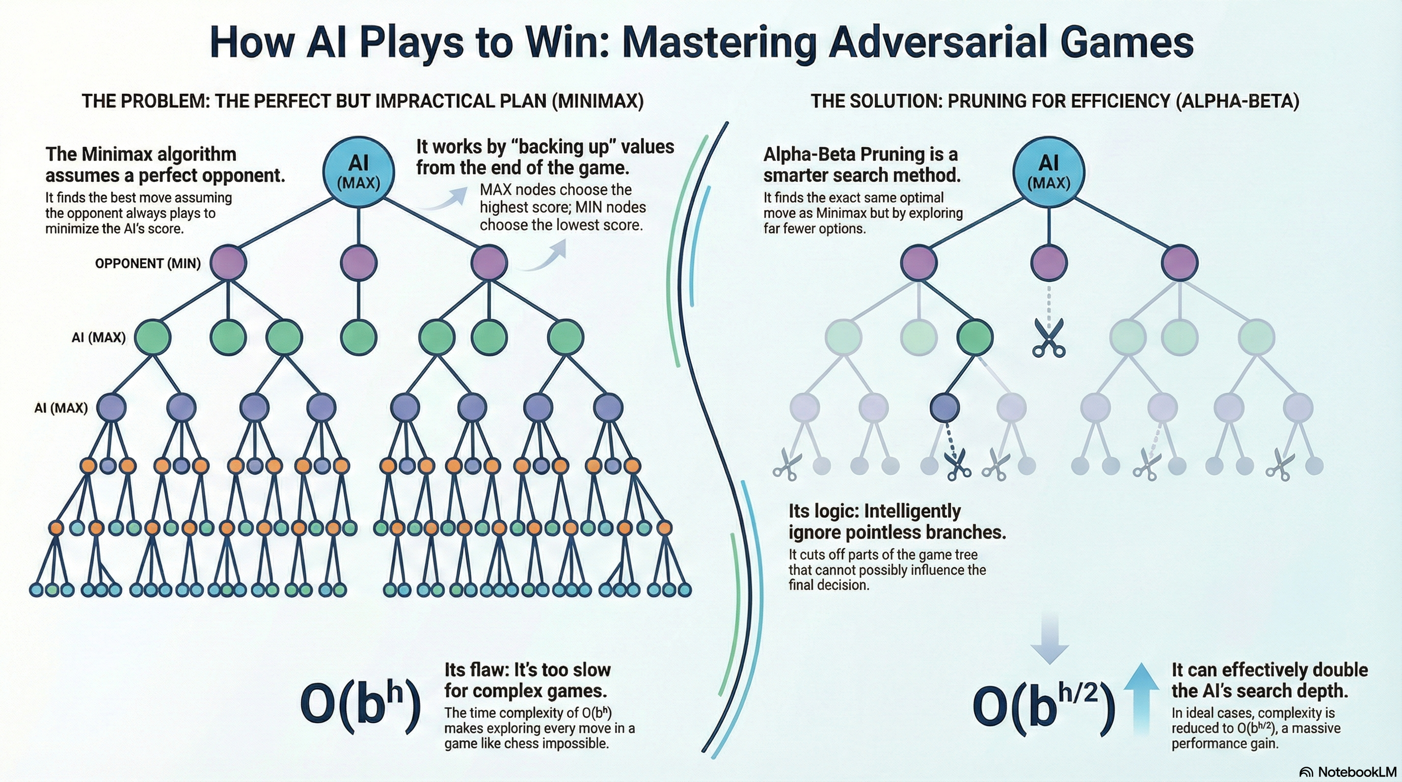
In the study of Artificial Intelligence, adversarial search addresses a distinct and complex class of problems situated within multi-agent environments where agents possess conflicting objectives. This domain moves beyond simple optimization problems against a static environment and into the realm of dynamic strategic decision-making. In this context,
an agent's success is contingent not merely upon its own sequence of actions, but upon its ability to anticipate and counteract the strategies of one or more intelligent opponents.
The quintessential examples of such scenarios are deterministic, turn-taking games like Chess or Go, where the environment is not passive but actively antagonistic. The fundamental challenge, therefore, is to develop a policy—a strategy for choosing moves—that is robust against a rational opponent who is also trying to optimize their own outcome, often at our agent’s expense.
Characteristics of Adversarial Games
To develop foundational algorithms, analysis is initially confined to a specific category of games defined by a shared set of simplifying properties. These characteristics create a controlled environment for developing and understanding core search techniques. The games under consideration are typically two-player, where for convention we designate our agent as
- MAX’s objective is to reach a game state with the highest possible utility, while
- MIN’s objective is to force a state with the lowest possible utility.
The game proceeds in a turn-taking fashion, with players alternating their moves.
A critical assumption is that these games are zero-sum, which formalizes the purely competitive nature of the interaction. In a zero-sum game, the total utility across all players is constant, meaning any gain for one player is a corresponding loss for the other.
For a terminal state
Finally, the games are assumed to be deterministic, where the result of applying a move to a state is a single, uniquely determined successor state. This removes the element of chance. While many popular games like Backgammon incorporate stochastic elements (e.g., dice rolls), the fundamental algorithms of adversarial search are first developed for the deterministic case before being extended to handle uncertainty.
Formulating Games as a Search Problem
To enable computational analysis, a game must be formally defined as a search problem. This formulation adapts the structure of classical search problems but introduces components to manage the adversarial nature of the environment. The primary distinction is that the agent cannot construct a fixed sequence of actions to reach a goal, as the opponent’s choices introduce uncertainty into the search space.
Definition
The formal definition of a game encompasses the following elements:
- an initial state
representing the game’s starting configuration; - a
function identifying the agents; - an
function that returns the set of legal moves from a state ; - a
transition model that returns the state resulting from performing action in state . The conclusion of the game is determined by a terminal test,
, which returns true for terminal states (such as a checkmate in chess). Finally, a function provides a numerical value for a terminal state from the perspective of player . Take a look at the implementations here
In a zero-sum game, this can be simplified to a single function that returns the utility from MAX’s perspective, typically with values such as
This structure can be implemented programmatically, often using an abstract class Game to define the game’s interface. Specific games, such as Tic-Tac-Toe, would then be implemented as concrete classes that inherit this structure and provide the specific logic for actions, results, and utility calculations.
class Game:
    """An abstract base class for a turn-taking, two-player game."""
    def actions(self, state):
        """Return a collection of the allowable moves from this state."""
        raise NotImplementedError

    def result(self, state, move):
        """Return the state that results from making a move from a state."""
        raise NotImplementedError

    def is_terminal(self, state):
        """Return True if this is a final state for the game."""
        return not self.actions(state)

    def utility(self, state, player):
        """Return the value of this final state to a player."""
        raise NotImplementedError

def play_game (game, strategies: dict, verbose=False):
	"""Play a turn-taking game. 'strategies' is a (player_name: function) dict,
	where function(state, game) is the game) is used to get the player's move. """
	state = game.initial

	while not game.is_terminal(state):
		player = state.to_move
		move = strategies[player](game, state)
		state = game.result(state, move)

		if verbose:
			print('Player', player, 'move:', move)
			print(state)

		return state
The Game Tree
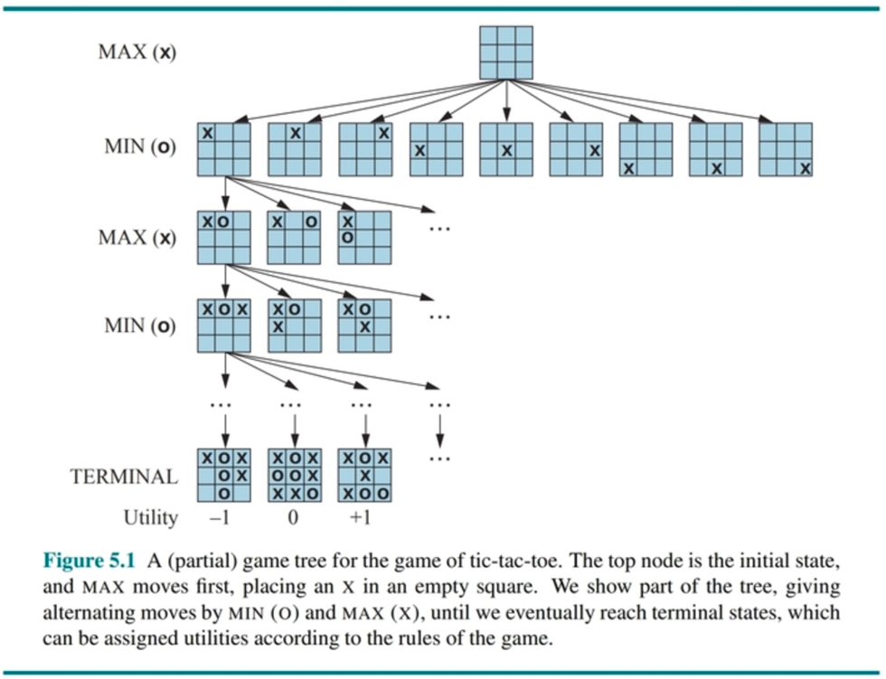
The concept of the game tree is a powerful abstraction for representing the dynamics of an adversarial search problem. This tree is a conceptual map of all possible sequences of moves, where each node corresponds to a unique game state and each edge represents a move.
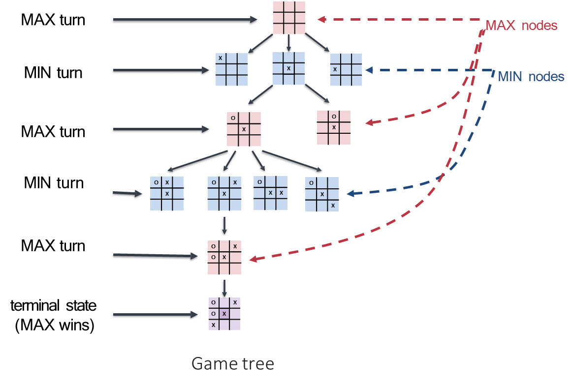
The root of the tree is the initial state from which the search begins. Its children are all the states reachable after one move, their children represent states reachable after two moves, and so on. The leaves of the tree are the terminal states of the game, where the outcome is definitively known.
A crucial feature of the game tree is that the players’ turns alternate with each level of depth, or “ply.” Levels where it is MAX’s turn to move are known as MAX nodes, and levels where it is MIN’s turn are MIN nodes.
Example
For games with a small state-space complexity, such as Tic-Tac-Toe, it is computationally feasible to generate this entire tree and thereby “solve” the game by finding a perfect strategy from any position.
The Minimax Algorithm
The fundamental challenge for complex games is to select the optimal move from the current state without exploring the entire game tree. The Minimax algorithm provides a foundational solution by formalizing the principle of optimal play against a rational opponent.
It determines the best move by assuming that the opponent will always choose the move that is most damaging to our agent.
seeks to maximize the final utility, while actively works to minimize it.
The algorithm performs a recursive, depth-first traversal of the game tree from the current state.
The algorithm operates as follows:
- Generate the Tree: Starting from the current state, generate the game tree down to the terminal states. (In practice, this is done via a depth-first search to a limited depth, but we first consider the full-tree case).
- Apply Utility: For each terminal (leaf) node, calculate its utility value from MAX’s perspective.
- Back Up Values: Propagate these utility values up the tree to the root. The value of a non-terminal node is determined by its children:
- The value of a MAX node is the maximum of its children’s values.
- The value of a MIN node is the minimum of its children’s values.
- Choose the Move: At the root node,
chooses the move (the edge) that leads to the child node with the highest backed-up value. This value is called the minimax value of the root state.
The
def minimax_search(game, state):
    """Search game tree to determine best move; return (value, move) pair."""

    player = state.to_move

    def max_value(state):
        if game.is_terminal(state):
            return game.utility(state, player), None

        value, move = -infinity, None

        for action in game.actions(state):
            value2, _ = min_value(game.result(state, action))
            if value2 > value:
                value, move = value2, action
        return value, move

    def min_value(state):
        if game.is_terminal(state):
            return game.utility(state, player), None
        value, move = infinity, None

        for action in game.actions(state):
            value2, _ = max_value(game.result(state, action))
            if value2 < value:
                value, move = value2, action
        return value, move

    if player == 'MAX':
        return max_value(state)
Example
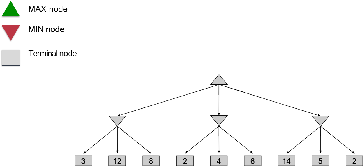
Consider a simple game tree where the terminal nodes have utilities of
for the first branch, for the second, and for the third.
- In the first step of backing up, the
nodes would take on the values - In the final step, the root
node would compute its value as . Therefore, the minimax value of the root is
, and the optimal action for is to make the first move, as it guarantees a utility of at least .
While the Minimax algorithm is provably optimal if it explores the entire tree, its computational complexity is its primary drawback. The time complexity is
For a complex game such as Chess, where
and a typical game depth , the number of nodes to evaluate is astronomically large, far exceeding the number of atoms in the observable universe.
The Need for Optimization: Pruning
The core inefficiency of the Minimax algorithm lies in its exhaustive exploration of every node in the search tree.
A significant portion of this search is often redundant, as it involves evaluating branches of the tree that a rational player would never actually choose. The necessity of exploring every node in the game tree results in an exponential time complexity of
, rendering it intractable for any non-trivial game like chess or Go.
The key insight for making adversarial search practical is that it is possible to compute the correct minimax decision without exploring these irrelevant subtrees. This process of intelligently ignoring portions of the search tree is known as pruning.
Example
To illustrate, consider a search in progress where
is evaluating its available moves. Suppose the evaluation of the first move reveals that it can guarantee a utility of at least 3, because has an option to limit the outcome to 3. Now, begins to evaluate a second possible move. The search proceeds down this new branch and finds a potential outcome of 2. This value is passed up to its parent node. At this moment, can make a critical deduction: comparing the first move, which guarantees a value of at least 3, with this new move, which so far appears to lead to a situation where the opponent (MIN) can force a value of at most 2. Since seeks to maximize its utility, it will never choose a path that leads to a value of 2 when a path leading to a value of 3 is already available.
Therefore, any further exploration of this second branch is futile; no matter how high the other outcomes in this branch might be,
will always choose the path leading to the value of 2. This entire subtree can be safely pruned, as it cannot alter the final decision at the root.
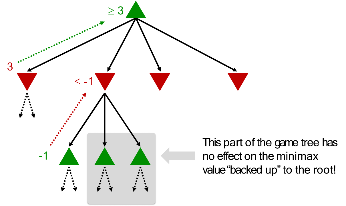
This logical shortcut forms the basis of the Alpha-Beta Pruning algorithm, a refined technique that maintains bounds on the outcomes and prunes any branch that is guaranteed to be suboptimal, dramatically improving search efficiency without compromising optimality.
Alpha-Beta Pruning
This algorithm functions as a significant optimization to the Minimax search process by systematically eliminating, or “pruning,” large portions of the search tree that cannot possibly influence the final decision. Crucially, this is not an approximation;
Alpha-Beta Pruning is guaranteed to yield the exact same optimal move as a full Minimax search, but by exploring a potentially much smaller subset of the game state space.
The efficiency of Alpha-Beta Pruning is derived from maintaining two values, alpha (
- The alpha value, associated with the maximizing player (
), represents the best (highest) score that can ensure for itself, given the portion of the tree explored so far. It functions as a lower bound on the final outcome, initialized to negative infinity, and is only ever updated to a higher value. - The beta value, associated with the minimizing player (
), represents the best (lowest) score that can hold to. It acts as an upper bound on the outcome from ‘s perspective, initialized to positive infinity, and is only ever updated to a lower value.
Together,

The central principle of the algorithm is the pruning condition: if at any node, alpha becomes greater than or equal to beta (
), the subtree rooted at that node can be pruned. This condition signifies that the current path being explored cannot lead to a better outcome than one already discovered.
The logic is best understood from the perspective of a node’s parent. If a
function ALPHA-BETA-SEARCH(game, state) returns an action
	player ← game.To-MOVE(state)
	value, move ← MAX-VALUE(game, state, -∞, +∞)
	return move

function MAX-VALUE(game, state, α, β) returns a (utility, move) pair
	if game.Is-TERMINAL(state) then
		return game.UTILITY(state, player), null
	v ← -∞
	for each a in game.ACTIONS(state) do
		v2, a2 ← MIN-VALUE(game, game.RESULT(state, a), α, β)
		if v2 > v then
			v, move ← v2, a
			α ← MAX(a,v)
		if v ≥ β then return v, move
	return v, move C

function MIN-VALUE(game, state, α, β) returns a (utility, move) pair
	if game.Is-TERMINAL(state) then return game.UTILITY(state, player), null
	v ← ∞
	for each a in game.ACTIONS(state) do
		v2,a2 ← MAX-VALUE(game, game.RESULT(state, a), α, β)
		if v2 < v then
			v, move ← v2, a
			β ← MIN(β,v)
		if v ≤ α then return v, move
	return v, move
Example
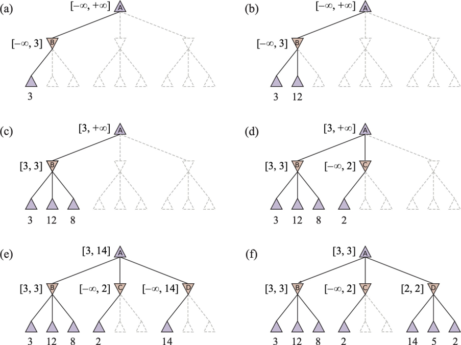
Consider the following example where Alpha-Beta Pruning is applied to a simple game tree. The pruning process is illustrated step-by-step, showing how branches of the tree are eliminated based on the alpha and beta values.
As we have done for the Minimax algorithm, we use the following conventions to represent the game tree:
(Upward Triangle): A Maximizing node (MAX). It wants the highest score. It maintains Alpha ( ), the minimum score it is guaranteed to get so far. (Downward Triangle): A Minimizing node (MIN). It wants the lowest score. It maintains Beta ( ), the maximum score it is guaranteed to get so far. We have to introduce two new values,
and , to keep track of the best scores that the two players can guarantee at any point in the tree. We initialize them as follows:
Pruning Rule: If at any point
, we stop searching that branch (prune it). This means the Maximizer already has a better option elsewhere, or the Minimizer already has a better option elsewhere, so this current path is irrelevant.
Step (a): Traversing the First Branch
- Start at A (MAX): The algorithm starts at the root. The search window is
. - Go to B (MIN): We descend to the first child, B. B inherits the window
. - Visit Leaf 3: B visits its first child, which has a value of 3.
- Update B: Since B is a Minimizer, it wants the smallest value. It sets its current bound (
) to 3.
- State: Node B now knows its value will be at most 3.
- Range at B: Updated to
. Step (b): Continuing in Node B
- Visit Leaf 12: B visits its next child, value 12.
- Comparison: B compares 12 with its current best (
). Since B is a Minimizer, it ignores 12 because . - No Change: B’s constraint remains at most 3.
Step (c): Finishing Node B & Updating Root
- Visit Leaf 8: B visits its last child, 8. It is ignored because
. - Return to A: Node B has finished and returns the value 3 to parent A.
- Update A (MAX): A is a Maximizer. It compares the returned 3 against its current
(which was ).
- A takes 3 as its new guaranteed lower bound.
- Update
: . - New Range at A:
. - Meaning: “I (Node A) am now guaranteed to get a score of at least 3. I will not accept any branch that yields less than 3.”
Step (d): Pruning at Node C
- Go to C (MIN): A moves to the next child, C. It passes down the current window
. This tells C: “Only bother reporting back if you can find a value greater than 3.” - Visit Leaf 2: C visits its first child, value 2.
- Update C: C is a Minimizer. It sets its temporary value to 2.
- C’s internal range becomes
. - The Pruning Logic:
- Parent A requires
(Alpha). - Node C has found a 2. Since C is a Minimizer, its final value can only go down (be 2 or less). It can never reach 3.
- Conflict:
(Alpha) (Beta). - Action (
CUT): The algorithm prunes the rest of C’s children.
- We do not visit the other children of C (shown as dashed lines). A will never choose path C because getting a 2 is worse than the 3 it already has from path B.
Step (e): Traversing Node D
- Go to D (MIN): A moves to the final child, D. It passes down the window
. - Visit Leaf 14: D visits its first child, 14.
- Update D: D updates its
to 14.
- Check Pruning: Is
? No. - Meaning: 14 is a valid possibility for A (since
), so we must continue searching D to see if it finds a smaller number. - Range at A: The image temporarily updates A’s visual range to
, showing that the best outcome currently possible on this path is 14. Step (f): Finalizing
- Visit Leaf 5: D visits the next child, 5. Minimizer D prefers 5 over 14.
- Update
to 5. - Check Pruning: Is
? No. Continue. - Visit Leaf 2: D visits the last child, 2. Minimizer D prefers 2 over 5.
- Update
to 2. - Check Pruning: Is
? Yes. (If D had more children, we would stop now. Since it’s the last child, we just finish). - Return to A: D returns the value 2.
- Final Decision at A: A compares its current best (
) with the returned value (2).
. Max prefers 3. - A keeps the value 3.
- Result: The best move is to choose branch B.
Summary of Updates
- Step (a-c): B finds min(3, 12, 8) = 3. A updates
to 3. - Step (d): C finds 2. Since
(Alpha), we PRUNE immediately. - Step (e-f): D finds min(14, 5, 2) = 2. A compares 3 vs 2 and keeps 3.
The performance gains achieved by Alpha-Beta Pruning are profoundly dependent on the order in which moves are evaluated.
- In the worst-case scenario, where the algorithm consistently explores the least optimal moves first, no pruning will occur, and its performance degenerates to that of the full Minimax search.
- In the ideal case of optimal move ordering, where the best possible move from any state is always examined first, the algorithm’s effectiveness is maximized. Under these conditions, the time complexity is reduced to approximately
.
This exponential improvement is transformative; it implies that with the same computational resources, an AI can search roughly twice as deep into the game tree, significantly enhancing its strategic capabilities. In practice, perfect ordering is rarely achievable, but heuristics can be used to sort moves based on their promise before a deep search, allowing the algorithm to approach this optimal performance.
Practical Implementations in Resource-Constrained Environments
Even with the optimizations of Alpha-Beta Pruning, searching to a terminal state in complex games remains computationally impossible. Practical game-playing agents must therefore operate within finite resource limits, primarily time. The standard approach to manage this is to employ a depth-limited search, where the algorithm only explores the game tree to a predetermined maximum depth, or “horizon.” Nodes at this depth limit are treated as terminal leaves, even though the game is not over.
This raises a new challenge: since these nodes are not true terminal states, their utility cannot be definitively calculated.
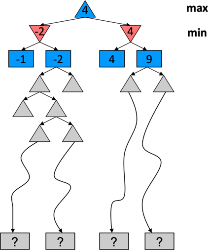
This limitation necessitates the use of a heuristic evaluation function, denoted
For instance, a simple evaluation function for chess might calculate the material advantage based on the pieces each player has on the board.
More sophisticated functions are typically structured as a weighted linear sum of various features (
The use of a depth limit and a heuristic evaluation function is not without its flaws. It can lead to strategic errors, most notably the horizon effect, where an agent makes a move to delay an unavoidable negative consequence just past its search depth, creating a false sense of security. However, there exists a fundamental trade-off between search depth and the complexity of the evaluation function.
A more accurate but computationally expensive evaluation function restricts the achievable search depth, while a faster, simpler function allows for a deeper search. Deeper searches can often compensate for minor inaccuracies in the evaluation, as the consequences of moves become clearer further down the tree. Finding the optimal balance between these two components is a central challenge in the design of high-performance game-playing AI.
Handling Uncertainty
While deterministic games provide a clear framework for introducing adversarial search, many real-world competitive scenarios involve an element of chance. These stochastic games, which include dice rolls in backgammon or card shuffles in poker, require an extension of the Minimax paradigm. To model such environments, the traditional game tree is augmented with a third type of node: the chance node. These nodes represent random events that are not controlled by any agent, and their outcomes are governed by a known probability distribution. The inclusion of chance fundamentally alters the objective from preparing for a perfectly rational opponent’s best move to optimizing for the best expected outcome across all possibilities.
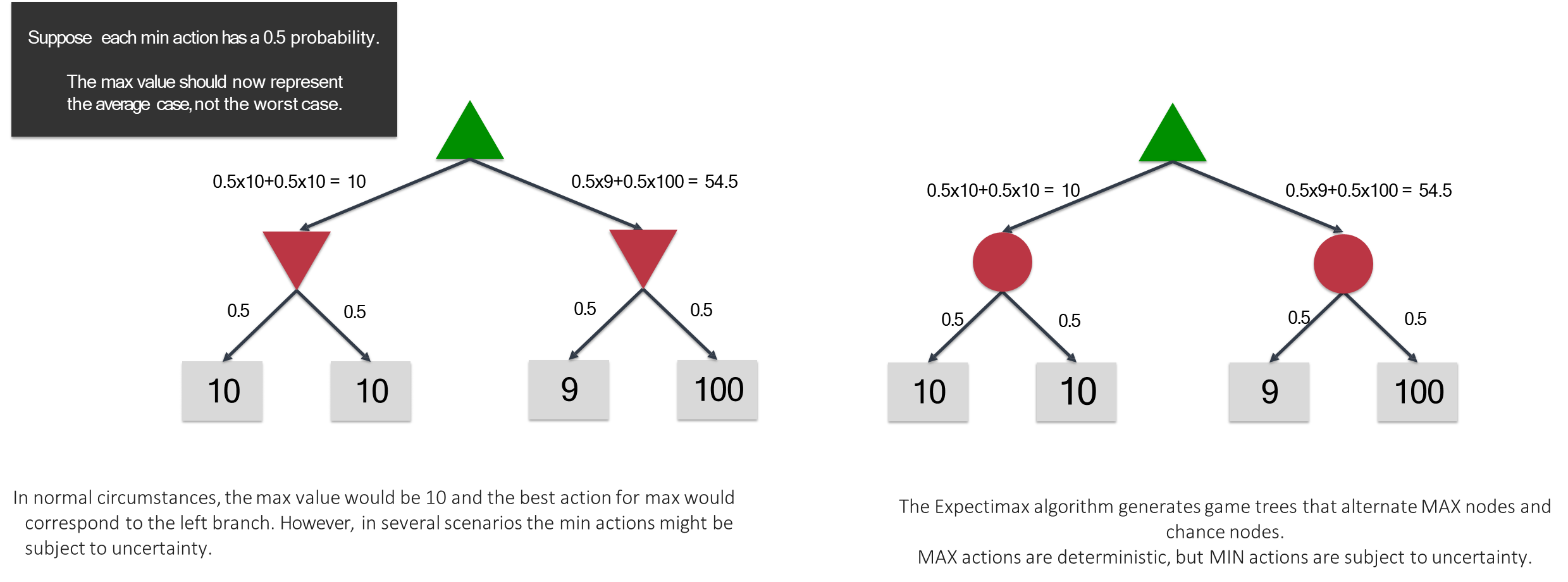
This shift in objective leads to the Expectiminimax algorithm, a variant of Minimax designed for games that incorporate
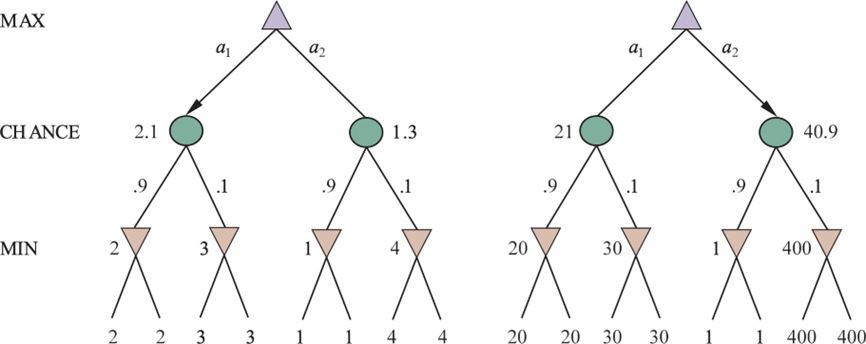
This approach ensures that the agent’s strategy is robust and optimized for the most likely series of events, rather than being overly conservative by focusing solely on the worst-case scenario which may have a very low probability of happening.
Because the algorithm computes weighted averages, the absolute magnitude of the utility values becomes critically important. A low-probability outcome with an exceptionally high payoff can significantly influence the expected value of a move, potentially making it the optimal choice over a more conservative option with a guaranteed but lower payoff. Consequently, the utility function must accurately reflect the true desirability of different terminal states, as its scale directly impacts the strategic decisions made by the algorithm.
Pruning and Practical Considerations in Stochastic Search
Alpha-Beta Pruning can be adapted for use in Expectiminiminax search, but its application is more complex and generally less effective than in deterministic games.
To establish the bounds necessary for pruning, the algorithm must have knowledge of the minimum and maximum possible utility values in the game. Even with this information, pruning is only possible in more limited circumstances, such as when the best-case expected value of a subtree is still worse than an alternative path for
The probabilistic nature of chance nodes makes it difficult to establish the firm bounds that allow for aggressive pruning. However, the impact of this reduced pruning efficiency is somewhat mitigated by the nature of stochastic games themselves. The probability of reaching any specific deep node in the tree diminishes with depth, meaning that errors introduced by a depth-limited search and heuristic evaluation functions are often less severe, as the far-future states they evaluate are less likely to be realized. This makes the trade-off between search depth and evaluation accuracy a central, yet manageable, challenge in developing agents for stochastic adversarial environments.