9 - Uncertainty

---

The Inevitability of Uncertainty in AI

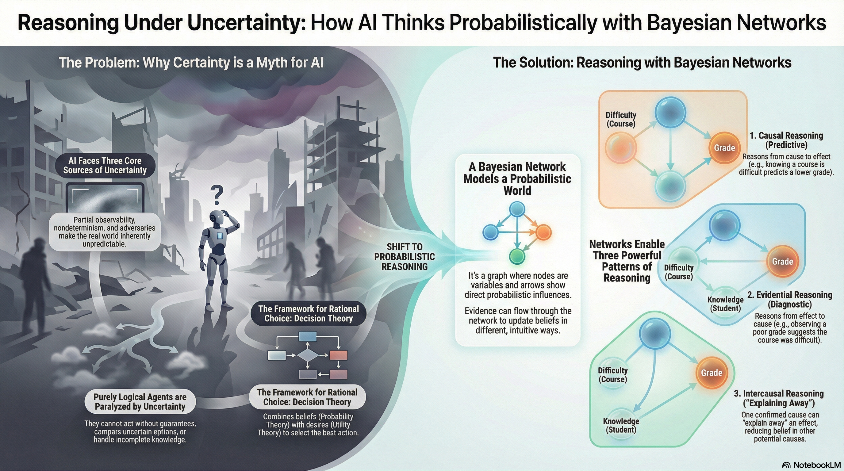
An intelligent agent operating within a real-world environment, as opposed to a purely simulated or idealized one, must invariably confront and manage uncertainty. This necessity fundamentally distinguishes real-world agents from those designed for environments that are fully specified and deterministic, such as a rudimentary game of tic-tac-toe. In essence, real-world agents are almost universally denied access to a complete and perfectly accurate model of the environment. This foundational challenge arises from several critical, interconnected factors that limit an agent’s knowledge and predictive power.

1. The first major source of uncertainty is partial observability. An agent’s sensory apparatus provides only a constrained, incomplete, and often noisy window into the state of the world. Consequently, the agent is compelled to infer the true state of the world based solely on this limited and imperfect data, a process that inherently introduces a degree of doubt.

2. A second significant factor is nondeterminism, where the outcomes resulting from an agent’s actions are not guaranteed to be consistent or precisely predictable. This means the same action, executed in the same initial state, can lead to a variety of different successor states. This characteristic mandates that agents consider a probability distribution over potential outcomes rather than relying on a singular, guaranteed result.

3. In many complex environments, an agent must interact with or contend against other agents whose objectives and goals are potentially in conflict with its own. Competitive scenarios, such as strategic games like chess or backgammon, or complex economic negotiations, involve an opponent whose actions and future intentions are unknown to the agent in advance. The agent must therefore anticipate and model the opponent’s strategy as a source of dynamic and unpredicted environmental change.

A purely logical agent, one that demands absolute certainty for decision-making, would thus be rendered practically paralyzed in the vast majority of real-world scenarios. The ability to formally represent and reason using probabilistic or fuzzy models of uncertainty is therefore a fundamental cornerstone of modern artificial intelligence.

From State to Belief State

To systematically confront the inherent uncertainty of the real world, intelligent agents must fundamentally shift their representational paradigm from tracking a single, definite world state to managing a belief state.

Definition

A belief state is formally defined as the set of all possible world states that an agent currently hypothesizes it might be occupying, given the complete history of its executed actions and subsequent sensory observations.

Instead of asserting, “I am definitively located in room ,” an agent utilizing this paradigm reasons probabilistically, holding a set of possibilities such as, “I am in either room or room .” The process of knowledge assimilation is achieved through belief state updating. As the agent acquires new sensor data it systematically eliminates from the belief set all previously possible world states that are inconsistent with this new, verifiable evidence. This mechanism allows the agent’s representation of the world to be dynamically refined, converging toward the true state of affairs as more evidence is accumulated.

The adoption of a belief state necessitates the formulation of a contingency plan, also referred to as a conditional plan. Unlike traditional planning in deterministic environments which yields a linear sequence of actions, a contingency plan is structured as a decision tree or policy. It explicitly specifies the appropriate action to be executed for every possible observation or contingency that might arise during the plan’s execution.

Example

A plan might stipulate, for example: “Move forward. If a wall is detected by the sensors, then turn left. If the path remains clear, then continue moving forward.” This conditional structure is vital for operating effectively in partially observable and non-deterministic environments, as it allows the agent to adapt its behavior in real-time based on the environmental feedback it receives.

While the concept of a belief state is an essential conceptual advancement, representing it as a simple, unweighted set of possibilities and attempting to govern its updates with classical formal logic introduces severe and often intractable drawbacks, particularly as the complexity and size of the environment increase.

Drawbacks of the Set-Based Belief State Representation

1. Combinatorial Explosion: The primary computational issue is the combinatorial explosion of the state space. An agent is theoretically compelled to consider every conceivable explanation for its sensor observations, irrespective of the explanation’s prior probability or likelihood. This indiscriminately inflates the belief state to an unmanageably large size with an overwhelming proportion of highly improbable, yet logically possible, scenarios.

2. Unwieldy Contingency Plans: The requirement for a correct contingency plan to account for every possible sequence of sensor observations creates exponential complexity. The sheer number of potential observation sequences can grow exponentially with time, rendering the complete plan arbitrarily large and computationally prohibitive to generate, store, and execute. The necessity to include actions for even the most highly unlikely contingencies further compounds the bloat of the planning structure.

3. Inability to Act Without Guarantees: A purely logical agent’s decision-making is often paralyzed when no course of action can be proven to guarantee the achievement of the goal. Because logical inference fundamentally deals with truth and falsehood (certainty), it offers no mechanism for action in scenarios where success is merely possible but not guaranteed. Yet, intelligent agents in the real world are routinely required to select an action even in the face of significant uncertainty.

4. Lack of a Mechanism for Comparison (Utility Theory): When multiple plans exist, none of which are guaranteed to succeed, a set-based belief state provides no methodology for comparative evaluation. To make a rational decision, an agent must weigh the probability of success against the magnitude of the reward achieved upon success.

The Failure of Purely Logical Reasoning in Uncertain Domains

The fundamental limitations of applying formal logic to uncertain domains are most starkly revealed in fields like medical diagnosis. The attempt to encode the causal relationship between a symptom and a disease, such as a and a , into a strict logical implication () immediately fails due to the fact that a toothache can be caused by numerous other conditions ().

Attempting to create an exceptionless rule is computationally and epistemologically infeasible:

• Complexity and the Qualification Problem: It demands an enormous, impractical effort to exhaustively list the complete set of necessary antecedents (causes) or consequents (effects) for every rule. This is known as the qualification problem, where it is impossible to list all necessary preconditions for a rule to hold true.

• Incomplete Knowledge: Most complex real-world domains, including medicine and biology, are not fully formalized or understood. A complete, exceptionless axiomatic theory of all diseases and their manifestations simply does not exist for the agent to model.

• Uncertain Evidence: Even if a complete set of logical rules did exist, the premise itself (the observation or evidence) is often uncertain. A patient’s diagnosis may remain uncertain because necessary diagnostic tests are either inconclusive, unavailable, or too invasive to perform.

Decision Theory

The acknowledged limitations of purely logical reasoning in uncertain environments necessitate a transition to a new, more robust framework for rational decision-making. An intelligent agent operating in the real world cannot simply search for a guaranteed sequence of actions that will definitively achieve its goal. Instead, the process must involve choosing actions by formally weighing the likelihood of various potential outcomes against the desirability or value of those outcomes. This foundational requirement leads directly to the concepts of utility theory and decision theory, which together constitute a formal methodology for making optimal, rational choices in the presence of risk and incomplete knowledge.

The Airport Problem

Consider the common planning scenario of navigating to the airport in time for a scheduled flight. The agent’s goal is timely arrival, and the problem involves coordinating travel over a fixed distance (e.g., ) with a chosen departure time (e.g., minutes prior to the flight).

A purely logical agent is immediately hampered by the non-deterministic nature of the real world. A definitive logical proof of success for the initial plan is impossible because the world is subject to unpredictable contingencies, such as highly unexpected traffic congestion, equipment failures like a flat tire, external events like a road-blocking accident, or unforeseen delays at airport security. The logical paradigm only permits actions that are guaranteed to succeed.

This highlights the fundamental trade-off: certainty versus cost. While a plan to leave hours in advance would virtually guarantee on-time arrival, this maximization of probability incurs an exorbitant cost—namely, hours of time wasted waiting, an outcome that is highly undesirable. The inadequacy of pure success probability as the sole criterion forces the agent to consider a crucial question: What are my preferences?

A rational agent must be able to formalize its preference for the ideal outcome (timely, low-stress journey) over undesirable outcomes (missing the flight) and costly ones (excessive waiting). This necessity points toward a framework where a numerical score, or utility, can be assigned to each potential resolution, allowing for the formal comparison of different plans based on their overall desirability. This model requires a dual perspective: a probabilistic model of the world (what is likely to happen) and a measure of the agent’s values (what the agent wants).

To successfully model and reason about the agent’s inherent preferences, AI leverages utility theory.

Definition

Utility theory serves as a robust formal framework for reasoning about preferences by asserting that the desirability of any given final world state to an agent can be accurately captured by a single, real-valued number, which is its utility.

A core principle of rational action is that a rational agent is axiomatically defined as one that prefers states with higher utility. This mathematical representation makes preferences explicit, consistent, and, critically, computable.

By establishing a utility function that maps outcomes to numerical scores, the agent can explicitly evaluate the “goodness” of all possible terminal states.

For the airport scenario, this might be structured as a mapping from outcomes (e.g., missing the flight) to scores: a failure to meet the goal receives a highly negative utility (), an overly cautious but successful arrival receives a low positive utility (), and the optimal, timely arrival receives the maximum utility ().

While utility theory provides the necessary mechanism for quantifying value (desirability), it remains incomplete on its own. The agent must also know how likely each outcome is to occur given a specific action. This is where the framework of probability theory must be integrated to provide the necessary quantification of likelihood (uncertainty), setting the stage for Decision Theory.

The most rational and effective methodology for an intelligent agent to address uncertainty is through the formal synthesis of its beliefs (quantified by probabilities) and its desires (quantified by utilities).

Formula

The core relationship in this domain can be expressed as an axiomatic equation:

In this synthesized framework:

• Probability Theory furnishes the necessary mathematical tools to represent and dynamically update the agent’s beliefs regarding the likelihood of various possible world states and the outcomes of its actions, such as .
• Utility Theory provides the formal mechanism to represent the agent’s preferences and the subjective desirability assigned to those final outcomes, such as .

Rationality and the Principle of Maximum Expected Utility (MEU)

Within the paradigm of decision theory, a rational agent is defined as one that chooses an action designed to maximize its success on average, considering all weighted possibilities. This concept is formally captured by the Principle of Maximum Expected Utility (MEU).

Definition

The expected utility of a given action is the average of the utilities of all possible outcome states, weighted by their respective probabilities of occurrence. The mathematical definition for the expected utility of action is:

where:

• is the conditional probability that executing action will result in state , given the agent’s current percepts and accumulated evidence .
• is the utility assigned by the agent to the final outcome state .

The MEU Principle mandates that a rational agent must select and execute the action that achieves the highest expected utility among all available choices: .

The Maximum Expected Utility (MEU) principle provides a clear, actionable algorithm for designing an agent capable of selecting optimal actions in uncertain environments. The operation of a decision-theoretic agent can be summarized in a continuous, iterative loop encompassing state estimation, outcome prediction, and utility-based decision-making.

The agent maintains persistent internal knowledge, primarily a belief state (a probability distribution over possible world states) and a record of its last action.

Steps

The operational cycle is as follows:

1. State Estimation (Belief Update): Upon receiving a new sensory , the agent updates its internal . This update integrates the new evidence with the prior belief state, refining the probability distribution over the current state of the world.

2. Outcome Prediction: For every possible action, the agent utilizes its probabilistic model of the environment (the transition probabilities) to calculate the likelihood of reaching all potential successor states. This yields a set of outcome probabilities for each action, conditioned on the current .

3. Decision Making (MEU Calculation): The agent computes the expected utility for every contemplated action by combining the predicted outcome probabilities (from step 2) with its internal utility function (representing its preferences). It then selects the action that yields the highest computed .

4. Action Execution: The chosen optimal action is returned to be executed in the environment, completing the cycle and preparing the agent for the next iteration of perception and decision.

function DT-AGENT(percept) returns an action
    persistent: belief_state, probabilistic beliefs about the current state of the world
                action, the agent's previous action

    // 1. Update belief state based on new evidence
    update belief_state based on action and percept

    // 2. For each possible action, calculate expected outcomes
    calculate outcome probabilities for actions, given action descriptions and current belief_state

    // 3. Select the action with the highest expected utility
    select action with highest expected utility given probabilities of outcomes and utility information

    // 4. Return the chosen action to be executed
    return action

Bayesian Networks

The framework of Decision Theory, while providing a robust foundation for rational action under uncertainty, is fundamentally dependent on the agent’s ability to efficiently represent and compute with probabilities. A critical challenge arises from the intractability of representing the full joint probability distribution over all variables in any realistic domain.

For a domain characterized by binary (Boolean) variables, the complete joint distribution requires the storage of () probability values. This exponential complexity makes the full joint distribution computationally unmanageable for systems with more than a modest number of variables.

To overcome this computational bottleneck, a more compact and structured method is required to encode the probabilistic relationships among variables. This role is fulfilled by Bayesian networks, which leverage the inherent structure of the problem to achieve an efficient factorization of the joint distribution.

Definition

A Bayesian network is a directed acyclic graph (DAG) that serves to represent a joint probability distribution over a set of random variables. It offers an intuitive and highly structured way to model a probabilistic domain by explicitly detailing the conditional independence relationships between the variables.

The network is composed of three core structural and quantitative components:

1. Nodes and Variables: Each node in the graph corresponds to a distinct random variable within the domain.

2. Directed Edges and Dependencies: The directed edges define the probabilistic dependencies. An edge extending from node to node signifies that has a direct causal or influential relationship on . Consequently, is designated as a parent of , and is a child of .

3. Conditional Probability Tables (CPTs): Associated with every node is a Conditional Probability Table (CPT). This table quantitatively specifies the conditional probability distribution of given all possible configurations of its parent variables, denoted as . If a node has no parents (i.e., it is a root node), its CPT simplifies to its prior probability distribution, .

The foundational power of a Bayesian network lies in the explicit conditional independence assumptions embedded within its graphical structure. Specifically, the structure encodes the property that each variable is conditionally independent of its non-descendants, given the values of its parents. This crucial factorization assumption allows the complex full joint distribution to be computed as a simple product of the local CPTs:

This multiplicative decomposition, driven by the graphical representation of local dependencies, is the key mechanism that enables Bayesian networks to represent vast, complex probability distributions in a compact and computationally efficient manner, effectively solving the issue of combinatorial explosion.

Example

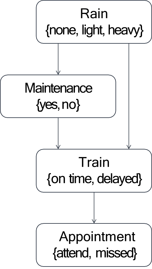
The construction of a Bayesian Network involves two systematic steps: first, defining the qualitative structure via the graph’s dependencies, and second, defining the quantitative parameters via the Conditional Probability Tables (CPTs). We will illustrate this process using the scenario of attending an appointment, where the outcome is subject to environmental and logistical factors.

The random variables in this domain are defined as follows:

• Rain (): The level of rainfall (possible values: ).
• Maintenance (): Whether track maintenance is being performed (possible values: ).
• Train (): The train’s status (possible values: ).
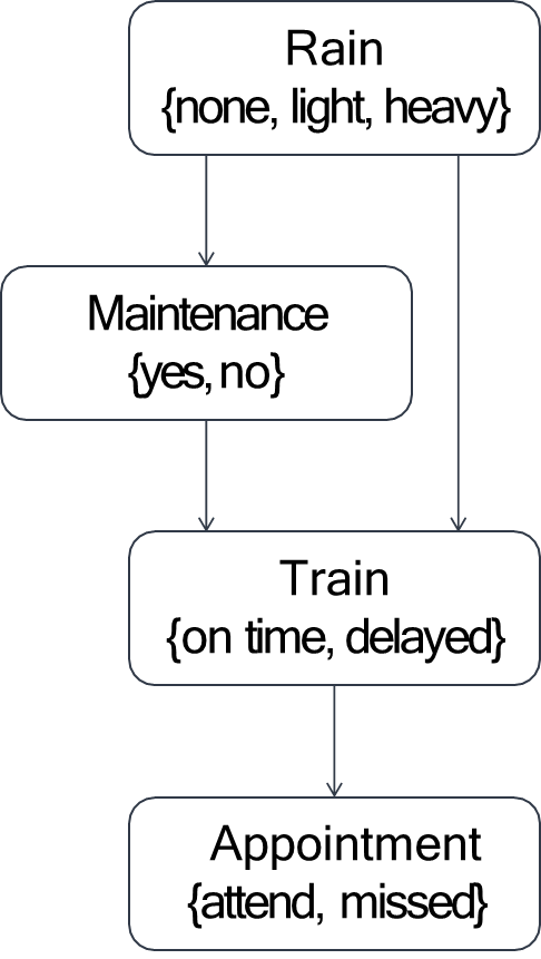
• Appointment (): The outcome of the appointment (possible values: ).

The graph structure is established by determining the direct causal or influential relationships between the variables. This step identifies the parent-child relationships, crucial for specifying the conditional independence assumptions.

1. Rain () is an exogenous (external) variable, not directly influenced by any other variable in the system. It is a root node.
2. Maintenance () is influenced by . For instance, may necessitate the postponement of scheduled . Thus, .
3. Train () status is directly affected by both (e.g., heavy downpour causes delays) and (e.g., track work causes delays). Thus, and .
4. Appointment () outcome is directly dependent on the ‘s status; a delayed train makes attending the appointment less likely. Thus, .

The second step involves quantifying the strength of the dependencies defined in the graph structure by providing the Conditional Probability Table (CPT) for each node.

As a root node with no parents, the CPT for is simply its prior probability distribution, .

	Probability
none	0.7
light	0.2
heavy	0.1

depends on , so we specify the conditional probability . Notice that the rows sum to for each condition of the parent variable .

Rain
none	0.4	0.6
light	0.2	0.8
heavy	0.1	0.9

The ‘s status depends on two parents: and . The CPT, , must enumerate all possible combinations of the parent variables.

Rain	Maintenance
none	yes	0.8	0.2
none	no	0.9	0.1
light	yes	0.6	0.4
light	no	0.7	0.3
heavy	yes	0.4	0.6
heavy	no	0.5	0.5
depends only on , so we specify .

Train
on time	0.9	0.1
delayed	0.6	0.4

With both the graph structure and the CPTs fully defined, the Bayesian network is complete. The network provides a complete and compact representation of the full joint probability distribution by factoring it into the product of the local conditional probabilities:

This factored representation significantly reduces the storage and computational requirements compared to storing the probability values required for the full joint table.

Computing Joint Probabilities with the Chain Rule

The principal advantage of a Bayesian Network is its capacity to facilitate the efficient calculation of the joint probability for any specific combination of events within the domain, without requiring the storage or manipulation of the exponentially large full joint probability table. This efficiency is achieved through the direct application of the Chain Rule for Bayesian Networks.

This chain rule is a direct consequence of the conditional independence relationships encoded in the network’s Directed Acyclic Graph (DAG). While the general product rule of probability states that , the structure of a Bayesian network allows for a powerful generalization. Because each variable is assumed to be conditionally independent of its non-descendants given its , the probability distribution is said to factorize over the graph .

Definition

The Chain Rule for Bayesian Networks formally states that the joint probability of a complete set of variables is the product of the conditional probability of each variable given only its direct parents in the network:

This formula mathematically asserts that the full joint distribution is entirely specified by the product of all the local entries found within the network’s small Conditional Probability Tables (CPTs).

Example

We can utilize this chain rule to compute the exact probability of a specific scenario using the previously defined network (Rain , Maintenance , Train , Appointment ). Let us calculate the probability of the specific event : Light rain (), no maintenance (), the train is delayed (), and the appointment is missed ().

graph LR
    R(Rain) --> M(Maintenance)
    R(Rain) --> T(Train)
    M(Maintenance) --> T(Train)
    T(Train) --> A(Appointment)

1. Decomposition by the Chain Rule: The joint probability is factored according to the network structure:

2. Substitution and CPT Lookup: We substitute the specific values of event into the factored expression:

3. Numerical Computation: By retrieving the corresponding numerical values directly from the CPTs:

   The resulting calculation is:

The probability of this specific conjunction of events is .

For a system with variables, this computation scales linearly with , providing a remarkable computational efficiency compared to the exponential storage and complexity of manipulating a full joint probability table.

Probabilistic Inference

A fully defined Bayesian Network transcends its role as a static probabilistic model; it functions as a dynamic computational engine capable of performing probabilistic inference.

Definition

Inference is the process of calculating the posterior probability distribution of a set of variables, given that the values of other variables in the network have been observed.

Fundamentally, inference enables the intelligent agent to update its beliefs (the prior probabilities) in a rigorously quantitative manner based on the reception of new evidence. To structure this process, the variables within the network are conceptually partitioned into three distinct sets relevant to a given query:

1. Query Variable (): This is the variable or set of variables whose posterior probability distribution is the objective of the computation. The agent is seeking to answer, “What is the probability of ?”
2. Evidence Variables (): This is the set of one or more variables in the network whose values are known or observed. The specific observed instantiation of these values is denoted by the vector .
3. Hidden Variables (): This set comprises all remaining variables in the network that are neither part of the query nor the evidence. Although unobserved in the current context, these variables are crucial because they form the internal probabilistic pathways that connect the evidence to the query variable, and their influence must be mathematically accounted for.

The ultimate computational goal of inference is to determine the posterior probability distribution of the query given the evidence, expressed as .

Example

For a concrete illustration using the train network: if we observe that the train was delayed, and we wish to find the probability of heavy rain, the variables are categorized as follows:

• (Query):
• (Evidence): , with observation :
• (Hidden): and

Marginalization

The complexity of inference lies in the necessity of correctly handling the hidden variables (). These variables cannot simply be discarded, as they are integral to the probabilistic chain of causality linking the evidence to the query . The core mathematical technique for eliminating the influence of these unobserved variables from the computation is marginalization, often colloquially termed “summing out” or “integrating out” (in the case of continuous variables).

The principle is derived from the Law of Total Probability, which states that

the probability of an event can be obtained by summing the joint probability over all mutually exclusive and exhaustive outcomes of another variable .

For a discrete random variable , the generalized definition of marginalization is:

Definition

The probability distribution of a variable can be computed from the full joint distribution by summing over all possible values of the hidden variables :

Where the summation is performed over all instantiations of the hidden variables .

This fundamental principle is the cornerstone of probabilistic inference in Bayesian networks. It allows the agent to calculate the unnormalized joint probability of the query and the evidence, , by summing out all the hidden variables () from the full joint distribution, which itself is compactly represented by the product of the CPTs (the Chain Rule):

Once is found for all values of , the final posterior probability is calculated via Bayes’ rule: . This requires an additional normalization step, where acts as the normalization constant.

Inference by Enumeration

Inference by enumeration is a foundational, though computationally intensive, method for calculating the posterior probability distribution of a query variable given evidence. The process involves systematically marginalizing (summing out) all hidden variables from the joint distribution, which is itself efficiently calculated using the Chain Rule.

Example

Let us apply this method to the train network to answer the query: What is the probability distribution for the (), given that there is rain and maintenance ()?

• Query ():

• Evidence (): (or )

• Hidden ():

Our objective is to compute .

We express the query using the definition of conditional probability: .

To circumvent the direct computation of the marginal probability of the evidence, , which would require its own separate marginalization calculation, we introduce a normalization constant, . The initial focus is on computing the unnormalized joint probability for all possible values of . The final normalization step will ensure the computed probabilities sum to unity.

To find the unnormalized joint probability , we must sum out (marginalize) the hidden variable, (), over all its possible values ():

The summation is expanded to explicitly show the contribution of each possible state of the hidden variable . This effectively enumerates every complete, consistent state of the world that includes the query variable and the evidence:

Each term within this summation represents a specific joint probability, which must now be calculated using the Chain Rule for Bayesian Networks. For the scenario where ():

By looking up the numerical values from the CPTs:

The calculation is:

Similarly, for the scenario where ():

The unnormalized distribution is . We find the normalization constant :

Finally, the normalized posterior probability distribution for the Appointment is:

The agent concludes that, given light rain and no maintenance, the probability of attending the appointment is and the probability of missing it is .

This detailed example demonstrates that inference by enumeration is mathematically sound, as it sums over every consistent state of the world (including the hidden variables). However, the number of terms in the summation grows exponentially with the number of hidden variables, , making this approach computationally impractical for larger, more complex networks. More efficient inference algorithms, such as Variable Elimination, are necessary for practical applications.

Patterns of Inference in Bayesian Networks

Bayesian networks are highly versatile computational tools whose power extends far beyond mere calculation of joint probabilities. Their principal utility lies in their ability to model and execute various fundamental patterns of probabilistic reasoning by dynamically propagating the impact of new evidence through the network’s graph structure. While the directed edges conventionally represent causal relationships (i.e., cause effect), the inference process itself is not constrained by this directionality and can flow:

1. From Cause to Effect (Causal Reasoning)
2. From Effect to Cause (Diagnostic Reasoning)
3. Between Causes of a Common Effect (Intercausal Reasoning or Explaining Away)

To illustrate these distinct patterns of reasoning, we utilize a canonical example: the Student Network, which models academic performance and related outcomes.

Example

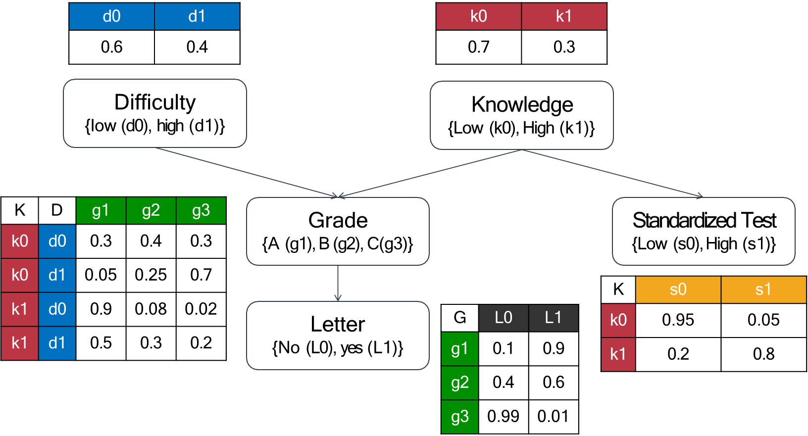
The Student Network models the probabilistic dependencies among factors that influence a student’s grade and subsequent outcome, such as the quality of a recommendation letter.

The network incorporates five random variables, all of which are discrete and have defined state spaces:

• Difficulty (): The inherent difficulty of the course, taking values in .
• Knowledge (): The student’s pre-existing knowledge or intelligence related to the material, taking values in .
• Grade (): The final grade received by the student, taking values in .
• Standardized Test (): The student’s score on a standardized exam, taking values in .
• Letter (): The quality of the recommendation letter written by the professor, taking values in .

The Graph Structure (Dependencies) is established based on logical causality:

• The student’s () is directly influenced by the course () and their intrinsic ().
• The student’s underlying () also directly influences their score on the ().
• The quality of the recommendation () is directly dependent upon the student’s () in the course.
• () and () are assumed to be independent root nodes; a course’s intrinsic difficulty is unrelated to the knowledge level of any single student.

According to the Chain Rule for Bayesian Networks, the full joint probability distribution for this five-variable system is factorized compactly as the product of the local conditional probability tables (CPTs):

The quantitative parameters that define the strength of the probabilistic relationships are provided alongside the graph. These CPTs, combined with the graphical structure, fully specify the Bayesian Network, enabling it to serve as a robust model for complex probabilistic inference.

Causal Reasoning

Causal reasoning, also frequently termed predictive reasoning or forward inference, involves predicting the likely effects when the causes are already known. In the context of a Bayesian Network, this type of inference flows in the same direction as the directed edges (i.e., from parent nodes to child nodes). This pattern allows the agent to update its belief about a descendant node based on evidence observed at an ancestor node.

Causal Inference Example: The Influence of Knowledge and Difficulty

We can analyze how evidence regarding a student’s intrinsic () and the course () predicts the likelihood of them receiving a ().

Inference Step	Query	Result	Observation
Prior Belief			This establishes the baseline probability without any specific information.
Posterior (K only)			Introducing the evidence decreases the probability of a strong letter, as low knowledge causally inhibits a good grade and, subsequently, a strong letter.
Posterior (K and D)			Introducing the additional evidence mitigates the negative impact of , increasing the probability of a strong letter by improving the expectation of the intermediate .

This sequence of calculations clearly demonstrates how causal evidence propagates downstream: a low cause () leads to a decreased effect, but a second, mitigating cause () can shift the prediction toward a more desirable effect.

The goal is to compute , using the shorthand notation , , and . The () is the hidden variable that must be marginalized out.

1. Conditional Probability and Factorization: We start by expressing the query as a marginalization over the hidden variable :

2. Applying the Chain Rule: We substitute the joint probability in the numerator with the factored product from the Chain Rule, :

3. Cancellation of Independent Terms (Important Simplification):

   Since and are independent root nodes, . More importantly, the terms and appear as common multiplicative factors in every term of the summation in the numerator, as they are not dependent on or . The term, while causally related to , is conditionally independent of given and can also be moved outside of the summation and then cancels (or is omitted if is not part of the evidence).

   A key realization for this specific causal pattern is that since the evidence is only at the parents of the query’s path, simplifies to a product of CPTs on the path.

4. Enumeration and Final Computation: We sum over the three possible grades :

   Plugging in the CPT values from (for ) and :

This result confirms that, when the course is easy, the low knowledge of the student is sufficiently mitigated to make a strong letter more likely than the prior belief, .

Diagnostic Reasoning

Diagnostic reasoning, also known as evidential reasoning or backward inference, involves the process of inferring the probable causes after having observed an effect. In a Bayesian Network, this type of inference flows against the direction of the causal arrows, propagating evidence from child nodes backward toward their parent nodes. This mechanism allows the agent to update its beliefs about the underlying factors responsible for an observed outcome.

Evidential Inference Example: Diagnosing the Grade

We examine how the observation of a () alters our beliefs concerning the two causal factors: () and ().

Query	Prior Belief	Posterior Belief	Observation
			The grade acts as an effect of the difficulty. The observation significantly increases the probability that the course was difficult, as this is a plausible diagnosis for the poor grade.
			The observation is strong evidence against the student having high knowledge. The probability plummets, confirming that low knowledge is a likely diagnostic explanation for the poor outcome.

Both calculations confirm that observing a negative effect () allows the agent to reason diagnostically, significantly increasing its belief in the negative causes () and decreasing its belief in the positive causes ().

The goal is to compute the posterior probability , using the shorthand and . This requires applying Bayes’ Rule and marginalization over the hidden variable ().

1. Application of Bayes’ Rule:

2. Marginalizing in the Numerator: We compute the joint probability by summing out the hidden variable over its states ():

3. Applying the Chain Rule to the Numerator: We expand the terms using the factorized joint distribution :

   Expanding the summation over () and ():

4. Numerical Computation of the Numerator: Plugging in the CPT values (, , ):

5. Final Calculation using Normalization: Assuming the prior marginal probability of the evidence is (as provided from the full network marginalization):

The resultant probability of confirms the strong diagnostic shift: observing a poor grade more than half-doubles the belief in the high difficulty of the course.

Explaining Away

The most sophisticated and complex form of probabilistic inference is intercausal reasoning, which arises in network structures where multiple independent causes converge upon a common effect. This structure, often termed a V-structure or collider, is critical because learning about the common effect (or any of its descendants) can introduce a probabilistic dependency between the initially independent causes.

The fundamental principle governing this pattern is known as “explaining away.” When the common effect is observed, and the presence of one cause is confirmed, the need for alternative causes to explain that effect diminishes. Consequently, the belief in the other potential causes decreases.

Explaining Away: The Grade Scenario (D G K)

In the , the () is the common effect influenced by the independent causes () and (). Prior to any evidence, and are independent: .

Question 1: Explaining a Poor Grade (G=C)

We observe the effect , which initially acts as negative evidence against the student’s ().

We then introduce the counter-evidence that the course was difficult (). This new fact provides an alternative explanation for the poor grade: the C could be due to the demanding nature of the course, not solely the student’s lack of knowledge.

Query	Belief Shift	Observation
		Baseline (Diagnostic): C strongly suggests low .
		Explaining Away: Knowing slightly increases the belief in . The difficulty explains away the , mitigating the negative diagnosis of the student’s knowledge.

Question 2: Explaining an Average Grade (G=B)

The principle is even more pronounced when the observed effect is less overwhelmingly negative, such as a .

Query	Prior/Diagnostic Belief	Posterior Belief	Observation
			Prior belief in high knowledge.
			Diagnostic: still slightly favors low over high .
			Strong Explaining Away: A in a difficult course () is strong positive evidence for the student. The high difficulty explains the B (which might be considered a poor grade if the course were easy), forcing us to conclude the student must have had high knowledge to achieve it. The belief increases significantly, even surpassing its prior.

This illustrates how the probabilistic relationships of the causes become coupled once information about their common effect is known.

Question 3: The Combined V-Structure and Evidential Flow

This scenario introduces evidence about a of one of the causes, specifically the () which is an effect of (). This highlights the power of the V-structure () combined with the causal link.

We observe: and .

1. Direct Diagnostic Inference (S K): The observation provides strong, independent, diagnostic evidence that the student must have .
   • was only .
   • . The positive evidence from overrides the negative evidence from .
2. Intercausal Reasoning (Explaining the Remaining Effect): Since we now strongly believe (the cause is present), we must explain why the common effect (the poor grade) occurred.
   • was .

The belief in the other cause, (), increases further. The strong knowledge (, inferred from ) has explained away the poor () as being due to the high difficulty of the course. This combined pattern of inference—evidence propagating up to a common cause (), and then intercausal reasoning coupling and at the common effect —is a complete demonstration of the sophisticated reasoning enabled by Bayesian Networks.

The phenomenon of intercausal reasoning or “explaining away” arises from the change in conditional independence relationships within a V-structure (or collider) when the common effect is observed. While the causes are initially marginally independent, conditioning on the common effect renders them conditionally dependent.

Example

To dissect this mechanism, consider a simplified probabilistic model featuring two independent causes, and , which jointly influence a common effect, .

For simplicity, let be determined by a stochastic OR function of and , where all combinations of the binary (Boolean) causes are equally probable a priori, .

​	​		Joint Probability
0	0	0	0.25
0	1	1	0.25
1	0	1	0.25
1	1	1	0.25

Initially, and are independent. The marginal probability of each cause occurring is (summing the last two rows). As required by independence, knowing ‘s state reveals nothing about ‘s:

Now, we introduce evidence by observing that the effect has occurred, . This observation fundamentally changes the sample space—the state is eliminated. The remaining three outcomes where are now the only possible states, and their total probability sums to . To perform inference, we normalize the probabilities of these remaining states so they sum to . Each of the three remaining rows now has a conditional probability of .

1. We first diagnose the probability of one cause given the effect:

The joint probability corresponds to the sum of the probabilities of the two rows where and (rows 2 and 4): .

The marginal probability of the evidence is the sum of probabilities of the last three rows: .

The observation has increased the belief in from its prior of to .

2. Next, we introduce the crucial piece of evidence: has occurred. We compute the conditional probability of given both the effect and the presence of the other cause: .

The new evidence eliminates the second row (). Only the rows where and remain (rows 3 and 4). The conditional probability is calculated over this further reduced sample space:

• (Row 4)
• is the sum of probabilities of rows 3 and 4:

Belief	Value	Change	Interpretation
Prior			Initial belief in cause .
Diagnostic			Observing the effect increases belief in the cause .
Intercausal			Observing that is present decreases belief in .

The comparison is less than . This is the fundamental, quantitative demonstration of explaining away: once the effect has been successfully attributed to the presence of the cause , the probability of the alternative cause reverts to its prior marginal probability (or often decreases further, depending on the CPT of ). The two causes, initially independent, are now conditionally dependent given the common effect, with knowledge of one cause attenuating the belief in the other.

Conditional Independence and the Flow of Influence

The fundamental utility of Bayesian Networks lies not only in performing complex computations but also in providing a graphical calculus for determining probabilistic relationships. The phenomena are all manifestations of influence flowing through the network structure. The key structural question addressed by this analysis is: When can we assert that two variables, and , are conditionally independent, given a third set of variables, ?

The answer is formalized by the concepts of active trails and d-separation, which offer a visual, graph-theoretic method for determining conditional independence.

Trail Structures

Definition

Any complete trail (a path regardless of arrow direction) between any two nodes and in a Bayesian Network can be decomposed into a sequence of only three fundamental three-node configurations.

Understanding how the flow of probabilistic influence is either active (transmitting influence) or blocked (preventing influence) through an intermediate node is the foundation of structural inference.

graph TD
	subgraph C[Common Effect]
		A3((X)) --> B3((W))
		C3((Y)) --> B3
	end

	subgraph B[Common Cause]
		B2((W))
		B2 --> A2((X))
		B2 --> C2((Y))
	end
	
	subgraph A[Causal Chain]
		direction LR
		A1((X)) --> B1((W))
		B1 --> C1((Y))
	end

1. Causal Chain (Serial Connection)

   • Structure:
   • Default Influence Flow: Active (Yes).
   • Mechanism: This is a standard causal chain where is a cause of , which is a cause of . Information about the root cause changes the belief about the intermediate variable (a predictive inference), which in turn modifies the belief about the final effect .

2. Common Cause (Diverging Connection)

   • Structure:
   • Default Influence Flow: Active (Yes).
   • Mechanism: Both and are effects of a common cause . This setup results in a marginal correlation between and . Observing initiates a diagnostic inference backward to the common cause , and the revised belief in then propagates forward to (a predictive inference).

3. Common Effect (Converging Connection / V-Structure)

   • Structure:
   • Default Influence Flow: Blocked (No).
   • Mechanism: and are independent causes of a single common effect . The intermediate node is referred to as a collider because the directed edges “collide” at this node. Crucially, in the absence of any evidence concerning (or any of its descendants), the two causes and remain marginally independent. Learning about provides no information about (e.g., the difficulty of a course tells us nothing about the student’s intrinsic knowledge). The trail is inherently blocked at the collider node by default.

This initial analysis leads to a preliminary but crucial structural rule for the flow of influence:

A trail between any two nodes, and , is capable of transmitting probabilistic influence if, and only if, it does not contain any colliders (V-structures).

A trail that satisfies this condition is designated an active trail in the absence of evidence.

Blocking and Unblocking Trails

The flow of probabilistic influence between any two variables and is fundamentally dependent on whether the intermediate node (or any node on the trail) is included in the evidence set (i.e., whether is observed). The introduction of evidence can either block an otherwise active trail or unblock an otherwise blocked trail, leading to the core principles of d-separation.

We re-examine the three basic three-node structures, now conditioned on observing ().

1. Causal Chain (Serial Connection):

   • Influence Flow when is Observed (): Blocked (No).
   • Rationale: If the exact state of the mediating variable is known, the variable provides no additional incremental information about the final effect . The influence of on is entirely channeled through . Once the value of is fixed by observation, the downstream probability of is fully determined by , making . Therefore, and are conditionally independent given .

2. Common Cause (Diverging Connection):

   • Influence Flow when is Observed (): Blocked (No).
   • Rationale: and are correlated because they share the common cause . However, once the state of is known, accounts for all the correlation between its two effects. Observing tells us nothing new about because the state of their common cause is already confirmed. Thus, and are conditionally independent given .

3. Common Effect (Converging Connection / V-Structure):

   • Influence Flow when is Observed (): Active (Yes).
   • Rationale: This is the critical, counter-intuitive case. As discussed in intercausal reasoning, and are marginally independent by default. However, conditioning on their common effect (or any descendant of ) unblocks the trail. This act of conditioning creates a dependency between and , which is the “explaining away” phenomenon. Learning that the effect is present requires its two causes to become coupled; confirming one cause () reduces the need for the other cause () to explain the observed effect.

Summary of Influence Flow Rules

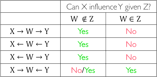
The rules for how evidence impacts the flow of influence are summarized below, defining when a trail is active or blocked.

Structure	W not Observed ()	W Observed ( or Descendant Observed)
Chains & Forks (→W→, ←W→)	Active (Transmits Influence)	Blocked (Stops Influence)
V-Structure (→W←)	Blocked (Stops Influence)	Active (Transmits Influence)

D-Separation and a Formal Definition of Active Trails

These graphical rules provide the basis for determining conditional independence in a Bayesian Network, formalized by the concept of d-separation.

Definition

Two nodes and in a Bayesian Network are d-separated by a set of evidence nodes if every single trail between and is blocked by . If and are d-separated by , then they are conditionally independent given , denoted as .

A trail between nodes and is classified as active given an evidence set if, and only if, the following two conditions are satisfied for every intermediate node along that specific trail:

1. Chains and Forks ( or ): The node must not be in the evidence set (). Observation of blocks these structures.
2. V-Structures (Colliders, ): The node or any of its descendants must be in the evidence set . Failure to observe the collider (or its descendant) blocks this structure.

If even one node along a trail violates these conditions, the entire trail is rendered blocked. The core task of d-separation is to inspect every possible trail between and to confirm that all of them are blocked by the evidence .

Trail in the Student Network

We will apply the rules of d-separation to a specific trail in the Student Network to formally determine the conditions under which probabilistic influence can flow.

The trail under examination is , which connects the () to the course ().

This trail involves two intermediate nodes with distinct structures:

1. Fork: At node ().
2. Collider (V-Structure): At node ().

For influence to flow between and , the entire trail must be active, meaning both intermediate nodes, and , must satisfy their respective active trail conditions for the given evidence set .

Scenario	Evidence Set ()	Analysis using D-Separation Rules	Can Influence Flow?
K is observed		Node K (Fork): Observed. Rule #1 states that observing a fork node blocks the trail ( is required for activity). The trail is blocked at .	No
G is observed		Node K (Fork): Not observed (), so this part of the trail is active. Node G (Collider): Observed (). Rule #2 states that observing a collider unblocks or activates the trail. Since both nodes are active, the entire trail is active.	Yes
Nothing is observed		Node K (Fork): Not observed (), so this part is active. Node G (Collider): Not observed (). Rule #2 states that not observing a collider blocks the trail. The trail is blocked at .	No

This formal analysis using d-separation rules perfectly corroborates the concept of intercausal reasoning or “explaining away” demonstrated earlier:

• In the absence of evidence (), and are d-separated (independent). The influence is blocked by the unobserved collider, . This confirms that knowing the intrinsic course difficulty tells you nothing about a student’s standardized test score unless you see their course grade.
• Conditioning on the common effect ( is observed) unblocks the trail. Learning the grade couples the two causes, and . Information flows from (evidence about ) through to and then through to . This allows the student’s test score to influence our belief about the course’s difficulty (e.g., a high test score combined with a low grade strongly suggests the course must have been very difficult).

Approximate Inference

The method of inference by enumeration provides an exact inference solution, guaranteeing the true posterior probability distribution for a query. However, its runtime complexity is exponential with respect to the number of variables in the network, rendering it computationally intractable for the large-scale networks found in many real-world applications.

To circumvent this severe limitation, we rely on approximate inference algorithms. These methods sacrifice the guarantee of an exact result for improved efficiency, providing a good estimate of the true probability that converges to the correct answer as computational time (and the number of samples) increases. The majority of approximate inference techniques are rooted in randomized sampling.

Sampling

The foundational concept of sampling is to replace complex, exhaustive probabilistic calculations over the entire distribution space with the generation of a large number of simulated samples or events. Each generated sample is a complete, single assignment of values to every random variable defined within the Bayesian network.

By generating a vast, empirical collection of these samples, the resulting dataset effectively creates a statistical approximation of the true joint probability distribution. Probabilistic queries can then be answered simply by counting the relative frequencies of the relevant events within this empirical dataset. The Law of Large Numbers ensures that as the total number of generated samples, , approaches infinity, the observed frequencies will converge to the true underlying probabilities.

Direct Sampling (Prior Sampling)

Direct sampling, or prior sampling, is the most straightforward method for generating these empirical events. This technique generates samples by systematically following the causal structure of the Bayesian network, moving strictly from the root nodes (causes) down toward the leaf nodes (effects).

Algorithm for Generating a Single Sample

1. Topological Sort: The variables are sampled in a topological order, ensuring that a node is sampled only after all of its parent nodes have already been assigned a value.

2. Sampling from Priors: For any root node (a node with no parents), a random value is drawn from its unconditional prior probability distribution, .

3. Sampling from Conditionals: For any subsequent node , a random value is drawn from its conditional probability distribution, , using the specific values that were already sampled for its parent nodes.

4. Completion: This process is repeated until a complete assignment of values to all nodes in the network, known as a complete sample , is achieved.

Single Sample from the Train Network

Using the structure :

• Sample (Rain): Draw from . Result: .
• Sample (Maintenance): Draw from the conditioned CPT . Result: .
• Sample (Train): Draw from the conditioned CPT . Result: .
• Sample (Appointment): Draw from the conditioned CPT . Result: .

The complete sample generated is . This process is iterated times to create the empirical dataset.

Once a sufficiently large set of samples has been generated, probabilistic inference is reduced to a straightforward counting exercise.

To estimate the probability of an event, , we count the number of samples in which the event occurs, , and calculate the ratio:

Example: Estimating

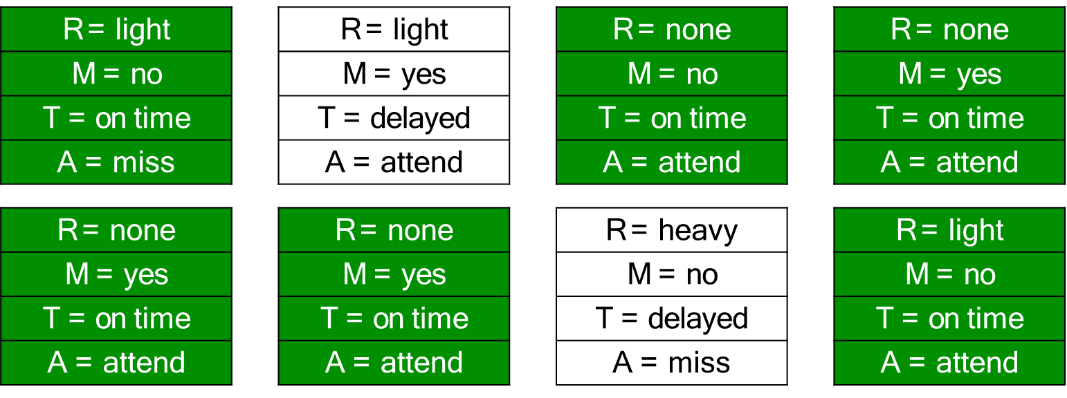
Given a dataset of samples (as provided in the table).

Sample	R	M	T	A	T = on time?
1	light	no	on time	miss	Yes
2	light	yes	delayed	attend	No
3	none	no	on time	attend	Yes
4	none	yes	on time	attend	Yes
5	none	yes	on time	attend	Yes
6	none	yes	on time	attend	Yes
7	heavy	no	delayed	miss	No
8	light	no	on time	attend	Yes

The count of samples where is .

The estimated probability is:

This sampling methodology avoids the computational complexity of the exact enumeration method. The primary trade-off is the accuracy of the estimate: higher accuracy requires a larger number of samples, thus increasing the linear complexity, but avoiding the exponential scaling of exact inference.

Rejection Sampling

Direct sampling (Prior Sampling) is effective for estimating prior probabilities like , but it cannot directly compute conditional probability queries of the form , where represents some observed evidence. To integrate this evidence into the sampling process, the simplest technique is Rejection Sampling. This approach uses direct sampling to generate a dataset and then systematically rejects any sample that is inconsistent with the observed evidence , thereby restricting the estimation to the relevant subset of the sample space.

The objective of rejection sampling is to estimate by restricting the population of samples to only those that match the evidence , and then using these remaining samples to count the frequency of the query variable .

Algorithm

1. Initialization: Initialize frequency counts for all possible values of the query variable to zero.
2. Sample Generation: Generate a large number of total samples, , using the standard Direct (Prior) Sampling algorithm.
3. Consistency Check and Rejection: For each generated sample :
   • Check Evidence: Determine if the sample is consistent with the observed evidence (i.e., if the values of all evidence variables in match the specified values in ).
   • Accept/Update: If the sample is consistent (accepted), increment the count corresponding to the value of the query variable found in .
   • Reject: If the sample is inconsistent (rejected), discard it and perform no updates.
4. Normalization: After processing all samples, estimate the posterior distribution by normalizing the final counts (dividing each count by the total number of accepted samples).

Rejection sampling mathematically simulates the definition of conditional probability:

Example: Estimating

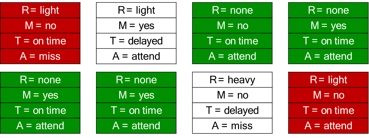
Using the provided 8 samples, we estimate the posterior probability of the query given the evidence .

We reject any sample where :

Sample					Consistent with T=on time?
1	light	no	on time	miss	Keep
2	light	yes	delayed	attend	Reject
3	none	no	on time	attend	Keep
4	none	yes	on time	attend	Keep
5	none	yes	on time	attend	Keep
6	none	yes	on time	attend	Keep
7	heavy	no	delayed	miss	Reject
8	light	no	on time	attend	Keep

Total number of consistent samples, , is .

We count the frequency of the query variable’s values within the 6 kept samples:

• Count for : (Samples 1, 8)
• Count for : (Samples 3, 4, 5, 6)
• Count for :

The estimated probability for is:

The estimated full posterior distribution for is

While rejection sampling is simple to conceptualize and implement, its principal and often fatal weakness is its extreme inefficiency in scenarios where the evidence is rare.

The inherent inefficiency stems directly from the method’s core principle: generating samples from the prior distribution and subsequently rejecting any sample that is inconsistent with the evidence . The problem becomes acute when the probability of the evidence, , is very small. In this case, the vast majority of computational time is wasted generating samples that are immediately discarded.

This represents an exponential waste of effort. For a query where the evidence is a rare or unlikely event—for example, a highly specific combination of symptoms leading to a diagnosis that occurs with a probability of —the agent would statistically need to generate, on average, one million total samples to obtain just a single sample consistent with the evidence. To achieve a statistically reliable posterior estimate, the required number of samples escalates quickly into the millions or billions, rendering the algorithm computationally infeasible for real-world, large-scale Bayesian Networks.

---

Applying Bayesian Networks - A Case Study in Medical Diagnosis

This chapter demonstrates the practical application of Bayesian Networks in a medical diagnosis setting, focusing on the steps required to model, represent, and perform inference regarding heart disease risk factors.

The objective is to construct a Bayesian Network utilizing the following six binary random variables:

• Exercise ():
• Diet ():
• Heart Disease ():
• Blood Pressure ():
• Heart Burn ():
• Chest Pain ():

The model must accurately reflect the causal relationships derived from expert medical knowledge.

Question 1: Modeling the Domain (Graph Structure)

The core task is to translate the qualitative statements provided by the physician into a Directed Acyclic Graph (DAG) by establishing the direct causal links between the variables.

graph TD
	E((Exercise))
	D((Diet))
	HD((Heart Disease))
	BP((Blood Pressure))
	HB((Heatburn))
	CP((Chest Pain))
	
	D --> HD
	D --> HB
	E --> HD
	HD --> BP
	HD --> CP
	HB --> CP

1. Diet’s Influence: “Unhealthy diet influences possible heart diseases and heartburn.” This establishes as a cause for two distinct effects:
2. Exercise’s Influence: “Regular exercise can limit problems of heart diseases.” This establishes as a cause influencing the primary disease variable:
3. Heart Disease and Blood Pressure: “High blood pressure can be an effect of a heart disease.” This defines the causal flow from disease to a physiological symptom:
4. Chest Pain Causality: “Patients can experience chest pain if they have heartburn but also if they have a heart disease.” This identifies as a common effect of two separate causes ( and ), creating a V-structure (or collider) at the node:

Combining these five causal links yields the complete DAG structure, which formally represents the joint probability distribution using the Chain Rule:

This structure defines the conditional independence assumptions of the medical domain: for instance, is dependent on , but is conditionally independent of and given .

Question 2: Calculating a Joint Probability

The task is to compute the joint probability of a specific partial state of the network:

This calculation utilizes the Chain Rule for Bayesian Networks, which allows the joint probability of any set of variables to be computed by factoring the full joint distribution into a product of local conditional probabilities defined by the CPTs.

The full joint distribution of the six variables () is:

Since the query involves only , and , and these four variables do not have any hidden variables or evidence descendants connecting them to or , the required joint probability is simply the marginalization of the full joint over the remaining variables (). Because the factorization inherently separates these groups, the necessary calculation simplifies to the product of the CPTs of the variables in the query:

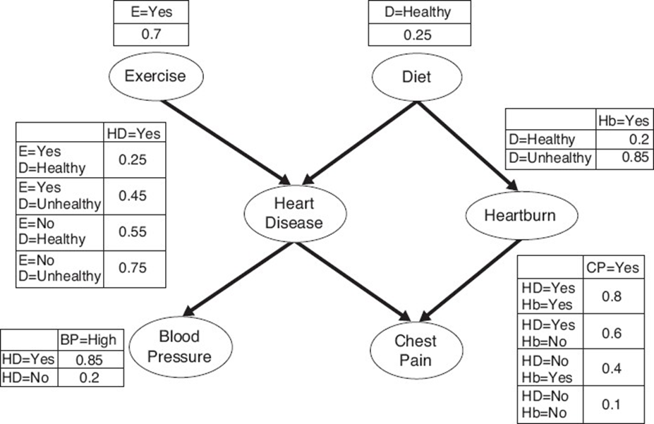
We plug the specific values from the query (, , , ) into the factored expression and look up the values in the provided CPTs:

1. Prior Probability of Exercise:

2. Prior Probability of Diet:

3. Conditional Probability of No Heart Disease: We need . The CPT provides .

4. Conditional Probability of High Blood Pressure:

The final joint probability is computed by multiplying the numerical values:

The probability of this specific scenario—a patient not exercising, having a healthy diet, not having heart disease, but still presenting with high blood pressure—is 0.675%. This demonstrates how the Bayesian Network, through the Chain Rule, allows for the efficient calculation of any joint probability using only the compact CPTs.

Further Queries

The remaining queries necessitate moving beyond simple joint probability calculations to full probabilistic inference. This requires accounting for the influence of unobserved variables through the mathematical operation of marginalization, or “summing out.” These examples demonstrate why the computational demands of exact inference by enumeration quickly become intractable in real-world Bayesian Networks.

Question 3: Marginalizing a Single Variable (Diet)

The query asks for the joint probability without specifying the patient’s (). thus becomes the hidden variable that must be marginalized over.

To obtain this marginal probability, we sum the joint probability over all possible states of the hidden variable , which are () and ():

Each term inside this summation is a specific joint probability that must be calculated using the Chain Rule (as shown in Question 2). The total computation requires two full joint probability calculations, demonstrating a simple increase in complexity due to the presence of a single hidden variable.

Question 4: Marginalizing Multiple Variables (P(ChestPain = Yes, HeartDisease = Yes))

This joint probability query, , is more complex as it requires marginalizing out four hidden variables (, , , ) which link the two query variables to the root nodes.

Since all four hidden variables are binary, the total summation requires separate terms to be calculated. Each of these 16 terms must be computed using the full Chain Rule of the network:

This exponential growth in the number of required computations clearly illustrates the intractability of exact inference by enumeration for even modestly sized networks.

Question 5: Marginalizing All Other Variables (P(BloodPressure = High))

This query asks for the prior probability of a non-root node variable, . This is the most computationally intensive type of prior probability query, as it requires summing out all five other variables ():

Since all six variables are binary, the summation must cover full joint probability terms. Each term requires a calculation using the complete Chain Rule.

These examples underscore the necessity of employing approximate inference methods, such as Likelihood Weighting or Gibbs Sampling, in practical applications. These sampling-based techniques provide computationally efficient estimates of the posterior probabilities, circumventing the exponential complexity associated with exact inference by enumeration.